4 Wrangling your data
We are now in the fourth week of the Spring 2022 semester. One quarter of the way through. Into February. Congratulations, y’all!
Today we’re going to start moving a little bit from abstract “how to” do things in R (but of course we’ll still have plenty of that) and into specific tasks that are relevant to food and ag scientists who need to do data science work. The focus today is going to be on
- Reading data into R (as well as a little discussion of how we store data)
- Learning to use
tidyverse, as set of R packages that makes R code easier and more intuitive (most of the time) - (If we have time), returning to functions, including how to make them (and your scripts) readable and useful
We’re going to have “the talk” about file extensions and how your computer stores data. Just like my discussion of data types in Week 1 (or, let’s be real, anything I do), this will be an informal and probably not 100% technically correct discussion. But learning to see these things properly will help you become a more capable user of scientific data.
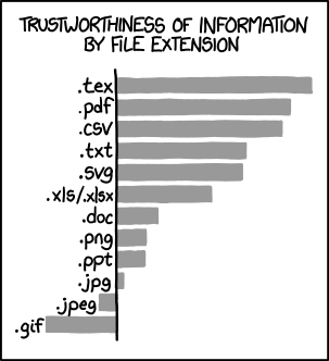
What file extensions can we trust? From XKCD.
4.1 Getting your data into R
One of the main challenges my students and others face in using R is getting data into the damn thing. I personally don’t think that most stats classes, or most classes on R, spend enough time on how to store your data, how to get it into a shape that R won’t struggle with too much, and how to actally get it into R (and what happens when you do).
I think one of the reasons for this is that typical software like SPSS or Minitab (or JMP) gives you a spreadsheet (Excel-like) interface to deal with your data, which you can either copy-paste in from Excel or input directly. Something like this:
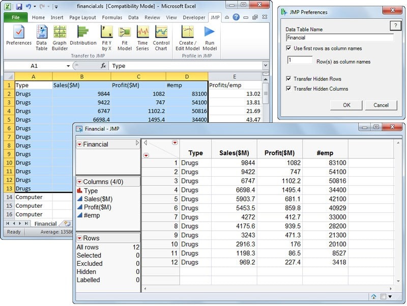
JMP’s interface directly imitates a spreadsheet, although it is not one.
In R, we have to use tools that are similar to the command line to deal with files. With some exceptions we will go over briefly, reading data into R follows the same rules we’ve learned about (in painful detail) so far: it is fast and powerful, but it also requires that we be very precise about how our data is stored already and how we want to bring the data into R.
These details seem arcane and pointless at first, and so we’re going to start by talking about how we store data in general.
4.1.1 Data storage outside R
Who here stores their lab notebook data in Excel? Raise your hand.
Me too! That’s because there’s nothing wrong with doing this (except that Excel is kind of a monster of a program, but that’s another story). Where we start running into problems is the intersection between data storage and data manipulation. Here is an example:
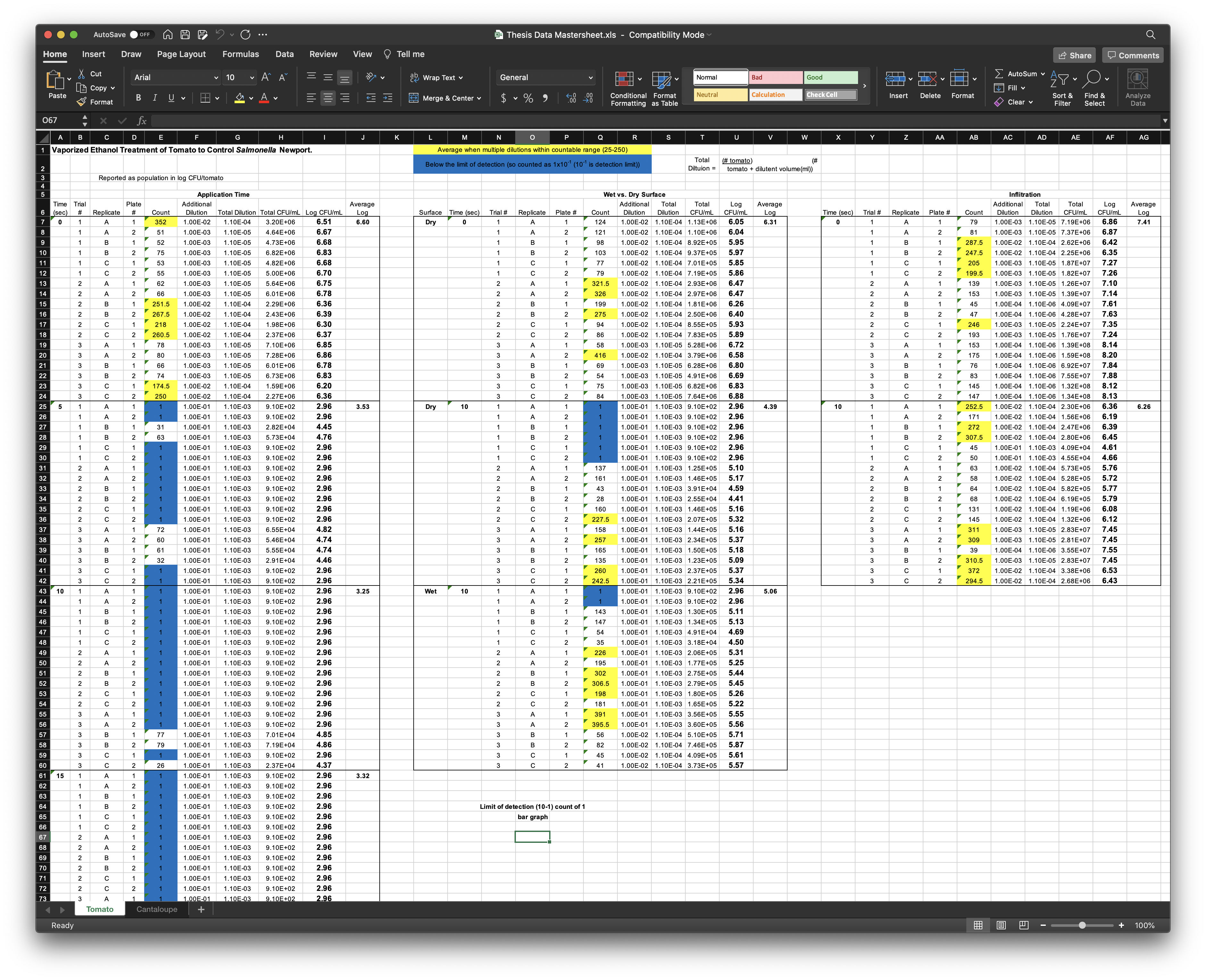
Michael Wesolowski’s thesis (2018) dataset uses Excel both to organize and to analyze data.
The problems with this approach are several-fold. First off, the analyses run in here (the average log calculation, for example), rely on the spatial alignment of the data. If the data are copy-pasted incorrectly, or a line is deleted, the analysis will become incorrect without giving any warning. Second, the visual annotation (the colored fields, the bolding, the outlines around cells) are not directly machine-readable (technically they are metadata that can be accessed with enough coding, but they are not directly attached to the data in a way that R or other programs can easily process).
But the worst thing about this well-organized lab notebook is that the data are organized in multiple columns and rows within the same sheet, and that there are informational headers and other notes throughout the sheet. The reason this is bad has to do with how computers (and R in particular) process files. In general, R is going to be expecting a file with consistent structure on each line.
Computers like structured data. Humans… may not. When we look at the above Excel file, our brains (which are pattern-finding engines) quickly intuit the patterns. We look to see where the colors are defined in the top lines, then check those out in the file. We understand that the first couple lines are “metadata”. But computers can’t know this (unless we build complex workflows for them to follow that encode that knowledge). So, instead, computers prefer data where the structure is predefined and there is no need for complicated rules.
The typical kind of data we will deal with in this class is delimited data. Non-rigorously defined, delimited data is data stored where each field is delimited by the same character. So, in the Excel file above, imagine that each cell value (A1, etc) is followed by the same character. This character could be anything, technically, but there are some conventional choices: comma-separated, tab-separated, or space-separated (least common). A comma-separated file would look like this:
# Comma-separated data

cat_acquisition_order,name,weight\n
1,Nick,9\n
2,Margot,10\n
3,Little Guy,13\n
This might look garbage-y, but let’s get in there. On each line of the file, we have three fields, each separated by a comma, and each line is ended (explicitly for the example) with the newline character: \n (the newline character is what your computer reads as “go to the next line”, like when you hit enter on your keyboard to go to a new line, you are explicitly entering a \n into the document).
One of the lines in this file looks like column names, whereas the rest look like a consistent pattern of data. So we can think of this as a way to represent tabular data in a plain-text file. In fact, comma-separated value files have their own, common file extensions: .csv. And they are one of the most common ways to read data into R, but it is by no means the only way–we will go over a few others below in the Why Data Storage is Hard section.
So how do we actually get these data into R? When we use JMP or SPSS or Minitab we can just open our .csv (or word file or whatever) and copy-paste the data into something that looks a lot like Excel. What happens if we try to copy-paste the cat example above into R?
In general, our workflow for R is the following:
- Store data in delimited format (usually .csv, but we will be talking about how to deal with existing Excel (.xls, .xlsx) files today as well.)
- Organize your file directories SOMEHOW
- Name your files usefully–if you’re not going to use git, it is a good idea to name files with dates (I like YYYYMMDD format).
- Use a function like
read.table()to read your data into R. - It makes sense to store your files (or a copy of your files) in the same folder as your R scripts
- If you want to use R to make changes to your files, use
write.table()or other functions to output your data back into the same folder. - THIS IS VERY IMPORTANT: Do not store data in R’s workspace. Your scripts/R Markdown files should always read in a data file, and make all changes to that file. This is why we clear changes on exit.
- We can store data in an R format using .RData files and the
save()function, but this makes the most sense only if we’re producing big or complex output we don’t want to rerun, and if we annotate the file well.
4.1.1.1 Example files
We are going to be working with several files in today’s example, which are all stored in the <class directory>/Files/Week 4/ directory on Canvas. You should store them in a similar format, although on your file system you’ll want to replace <class directory> with your actual directory structure. We’ll talk about directory structure very briefly later today.
The first file is polyphenol testing.csv, and it contains data from Sihui Ma’s dissertation (2019) research into polyphenols in apples. In this particular dataset, Dr. Ma was interested in the effect of readings of polyphenol content in response to different ratios of constituent polyphenols, because she suspected that tests were differentially responsive to different polyphenols (she was correct).
The second file is soup pilot data.csv. This is from research I conducted in 2016 at Drexel University on the effect of course order on acceptance for parts of a meal. This file, however, is just pilot data–we needed to develop different soups with different levels of base liking (outside of a meal), and so these are data from tasting of 4 soups, 2 minestrone and 2 hot and sour.
To start with, both of these files are well-structured. Here are some non-exhaustive attributes of that well-structuring:
- Each line is an observation.
- In the polyphenol file, that means each line is a single observation (this is long data).
- In the soup file, each line is a subject, with 4 observations (each soup) on the same line (this is wide data).
- There is no formatting or other non-readable information.
- The format of each file is 1 header line (names of variables) followed by each line as an observation that fits the pattern.
If your files are not in this format, it can sometimes make your life easier to get them into this format before you try to put them into R, although I will show at least one other option later.
4.1.2 read.table()
The most basic utitlity in R for reading in delimited data is the read.table() function. If you run ?read.table you’ll see that this is a function with a ton of options, because it is made to be very flexible and not assume a lot about the file you’re trying to read.
read.table(file = "Files/Week 4/polyphenol testing.csv",
           header = TRUE,
           sep = ",") # Note that this line tells read.table() how to break up your file - what happens if we exclude it with this file?
## Catechin PC.B2 Chlorogenic.acid equivalents.in.gallic.acid.mg.L
## 1 0.2 1 5 2.79
## 2 0.2 1 5 2.73
## 3 0.2 1 5 2.74
## 4 0.2 1 200 57.73
## 5 0.2 1 200 58.19
## 6 0.2 1 200 69.24
## 7 0.2 1 500 150.31
## 8 0.2 1 500 161.70
## 9 0.2 1 500 161.13
## 10 0.2 30 5 15.17
## 11 0.2 30 5 15.27
## 12 0.2 30 5 14.01
## 13 0.2 30 200 63.54
## 14 0.2 30 200 64.00
## 15 0.2 30 200 62.40
## 16 0.2 30 500 168.25
## 17 0.2 30 500 159.71
## 18 0.2 30 500 136.65
## 19 0.2 100 5 46.57
## 20 0.2 100 5 46.12
## 21 0.2 100 5 50.90
## 22 0.2 100 200 95.32
## 23 0.2 100 200 92.36
## 24 0.2 100 200 84.16
## 25 0.2 100 500 148.32
## 26 0.2 100 500 158.29
## 27 0.2 100 500 157.43
## 28 30.0 1 5 14.01
## 29 30.0 1 5 13.80
## 30 30.0 1 5 13.87
## 31 30.0 1 200 60.01
## 32 30.0 1 200 51.92
## 33 30.0 1 200 65.14
## 34 30.0 1 500 170.24
## 35 30.0 1 500 173.38
## 36 30.0 1 500 170.53
## 37 30.0 30 5 21.93
## 38 30.0 30 5 17.97
## 39 30.0 30 5 17.32
## 40 30.0 30 200 57.28
## 41 30.0 30 200 52.04
## 42 30.0 30 200 50.33
## 43 30.0 30 500 155.44
## 44 30.0 30 500 153.16
## 45 30.0 30 500 158.00
## 46 30.0 100 5 52.38
## 47 30.0 100 5 51.47
## 48 30.0 100 5 52.61
## 49 30.0 100 200 115.58
## 50 30.0 100 200 117.57
## 51 30.0 100 200 116.43
## 52 30.0 100 500 119.56
## 53 30.0 100 500 130.38
## 54 30.0 100 500 118.71
## 55 100.0 1 5 44.75
## 56 100.0 1 5 45.32
## 57 100.0 1 5 44.98
## 58 100.0 1 200 56.37
## 59 100.0 1 200 56.14
## 60 100.0 1 200 57.39
## 61 100.0 1 500 131.52
## 62 100.0 1 500 138.64
## 63 100.0 1 500 136.36
## 64 100.0 30 5 50.67
## 65 100.0 30 5 51.92
## 66 100.0 30 5 50.79
## 67 100.0 30 200 56.82
## 68 100.0 30 200 63.43
## 69 100.0 30 200 66.85
## 70 100.0 30 500 143.19
## 71 100.0 30 500 153.45
## 72 100.0 30 500 143.19
## 73 100.0 100 5 56.03
## 74 100.0 100 5 56.94
## 75 100.0 100 5 56.14
## 76 100.0 100 200 121.55
## 77 100.0 100 200 115.58
## 78 100.0 100 200 118.71
## 79 100.0 100 500 151.17
## 80 100.0 100 500 145.19
## 81 100.0 100 500 151.45The most important line here is the header = TRUE, which tells R that the first line in our file is a set of column names. Other options that are important are specifying the separator between columns (sep = "," tells this example that this is a .csv), and asis = TRUE, which will stop R from converting character data into factor data (the default behavior of read.table()).
We won’t necessarily be using read.table() very much, because more specific options like read.csv() or more general options like scan() will almost always be able to do what we want. But it is good to see the basic function in action. You’ll see read.table() come up a lot in older R scripts and references.
4.1.3 read.csv()
When we already know that the kind of data we’ll want to deal with is comma-separated, it’s much easier to use read.csv(), which does exactly what it sounds like. It is a wrapper function for read.table()–when you see something called a “wrapper”, it means it is actually just that function set up with some useful defaults. We can see that here:
read.csv## function (file, header = TRUE, sep = ",", quote = "\"", dec = ".",
## fill = TRUE, comment.char = "", ...)
## read.table(file = file, header = header, sep = sep, quote = quote,
## dec = dec, fill = fill, comment.char = comment.char, ...)
## <bytecode: 0x7fdd2776b4e0>
## <environment: namespace:utils>So read.csv() just tells read.table() a bunch of useful defaults so we don’t have to set them. Let’s try it on both of our files.
read.csv("Files/Week 4/polyphenol testing.csv")## Catechin PC.B2 Chlorogenic.acid equivalents.in.gallic.acid.mg.L
## 1 0.2 1 5 2.79
## 2 0.2 1 5 2.73
## 3 0.2 1 5 2.74
## 4 0.2 1 200 57.73
## 5 0.2 1 200 58.19
## 6 0.2 1 200 69.24
## 7 0.2 1 500 150.31
## 8 0.2 1 500 161.70
## 9 0.2 1 500 161.13
## 10 0.2 30 5 15.17
## 11 0.2 30 5 15.27
## 12 0.2 30 5 14.01
## 13 0.2 30 200 63.54
## 14 0.2 30 200 64.00
## 15 0.2 30 200 62.40
## 16 0.2 30 500 168.25
## 17 0.2 30 500 159.71
## 18 0.2 30 500 136.65
## 19 0.2 100 5 46.57
## 20 0.2 100 5 46.12
## 21 0.2 100 5 50.90
## 22 0.2 100 200 95.32
## 23 0.2 100 200 92.36
## 24 0.2 100 200 84.16
## 25 0.2 100 500 148.32
## 26 0.2 100 500 158.29
## 27 0.2 100 500 157.43
## 28 30.0 1 5 14.01
## 29 30.0 1 5 13.80
## 30 30.0 1 5 13.87
## 31 30.0 1 200 60.01
## 32 30.0 1 200 51.92
## 33 30.0 1 200 65.14
## 34 30.0 1 500 170.24
## 35 30.0 1 500 173.38
## 36 30.0 1 500 170.53
## 37 30.0 30 5 21.93
## 38 30.0 30 5 17.97
## 39 30.0 30 5 17.32
## 40 30.0 30 200 57.28
## 41 30.0 30 200 52.04
## 42 30.0 30 200 50.33
## 43 30.0 30 500 155.44
## 44 30.0 30 500 153.16
## 45 30.0 30 500 158.00
## 46 30.0 100 5 52.38
## 47 30.0 100 5 51.47
## 48 30.0 100 5 52.61
## 49 30.0 100 200 115.58
## 50 30.0 100 200 117.57
## 51 30.0 100 200 116.43
## 52 30.0 100 500 119.56
## 53 30.0 100 500 130.38
## 54 30.0 100 500 118.71
## 55 100.0 1 5 44.75
## 56 100.0 1 5 45.32
## 57 100.0 1 5 44.98
## 58 100.0 1 200 56.37
## 59 100.0 1 200 56.14
## 60 100.0 1 200 57.39
## 61 100.0 1 500 131.52
## 62 100.0 1 500 138.64
## 63 100.0 1 500 136.36
## 64 100.0 30 5 50.67
## 65 100.0 30 5 51.92
## 66 100.0 30 5 50.79
## 67 100.0 30 200 56.82
## 68 100.0 30 200 63.43
## 69 100.0 30 200 66.85
## 70 100.0 30 500 143.19
## 71 100.0 30 500 153.45
## 72 100.0 30 500 143.19
## 73 100.0 100 5 56.03
## 74 100.0 100 5 56.94
## 75 100.0 100 5 56.14
## 76 100.0 100 200 121.55
## 77 100.0 100 200 115.58
## 78 100.0 100 200 118.71
## 79 100.0 100 500 151.17
## 80 100.0 100 500 145.19
## 81 100.0 100 500 151.45read.csv("Files/Week 4/soup pilot data.csv")## subject minestrone1 minestrone2 hotandsour1 hotandsour2
## 1 1 0 50 -50 10
## 2 2 70 80 -20 20
## 3 3 80 97 10 37
## 4 4 20 60 -80 65
## 5 5 65 96 37 99
## 6 6 30 80 -50 20
## 7 7 75 90 40 80
## 8 8 70 80 50 -10
## 9 9 40 90 -60 20
## 10 10 15 65 25 20
## 11 11 -50 75 -15 50
## 12 12 75 25 -100 -100
## 13 13 -25 50 -75 -10
## 14 14 20 40 -75 60
## 15 15 70 90 -25 -60
## 16 16 20 90 -50 30
## 17 17 15 90 30 50
## 18 18 40 90 -60 -15
## 19 19 55 85 -50 -60
## 20 20 20 60 -40 0
## 21 21 20 100 -100 60
## 22 22 20 60 -60 -10
## 23 23 10 100 -100 85
## 24 24 10 75 35 55It’s been a little while since we did this, but what happens if we want that data?
polyphenol testing # We read the data and just threw it away!## Error: <text>:1:12: unexpected symbol
## 1: polyphenol testing
## ^Remember, we have to store R objects using <-.
polyphenols <- read.csv("Files/Week 4/polyphenol testing.csv")
soups <- read.csv("Files/Week 4/soup pilot data.csv")
Now we can access these objects and learn about them.
class(polyphenols) # the read.*() functions create data.frame objects## [1] "data.frame"head(polyphenols, n = 5) # display the first n lines of an object--defaults to n = 6## Catechin PC.B2 Chlorogenic.acid equivalents.in.gallic.acid.mg.L
## 1 0.2 1 5 2.79
## 2 0.2 1 5 2.73
## 3 0.2 1 5 2.74
## 4 0.2 1 200 57.73
## 5 0.2 1 200 58.19soups$minestrone1 # header = TRUE in read.csv() means that all the columns are named properly## [1] 0 70 80 20 65 30 75 70 40 15 -50 75 -25 20 70 20 15 40 55
## [20] 20 20 20 10 10And we can start to do basic data analysis. Let’s look at a boxplot of soup rating:
boxplot(soups[, -1]) # We use the [, -1] syntax to remove the first column of soups--why?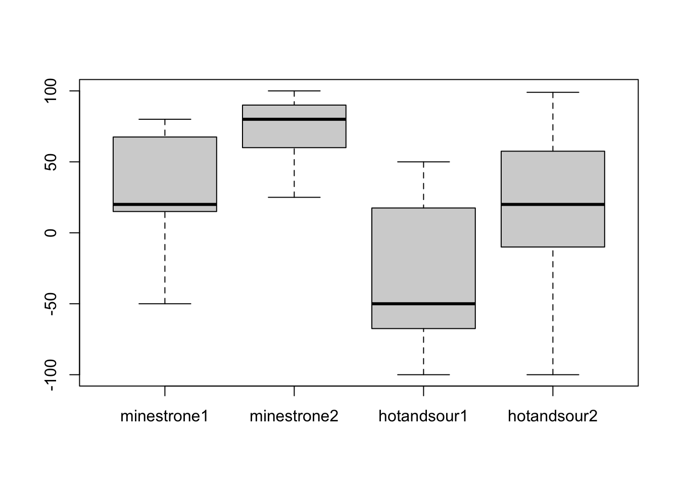
4.1.4 Why data storage is hard
OK, so we’ve pretty quickly gotten to getting data into R. That didn’t seem so bad. But let’s try importing a third file, which contains data from my lab from J’Nai Kessinger’s thesis (2019), in which she had subjects sort 18 ciders into groups according to their own perceptions. The file is called cider sorting.csv, but it has two problems.
- It is not stored in the standardized location I set up for this R Markdown
- It is well-formatted for human reading, but not for computers.
4.1.4.1 Where files live in your computer
The first problem above is one of file organization. Who here uses a set of structured folders to organize their files?
 But it seems like this is becoming less standard practice, according to this article in the Verge from Fall 2021. Both Windows and macOS have introduced more powerful search functions, so that if you have an idea of what your file is called you can kind of get away with just typing it into the search engine in the OS and having it return you the file.
Unfortunately, this plays pretty poorly with coding for research. We have a lot of data files that are often versioned–with the same file name but different dates. We also tend to have similar file names: “Cider ANOVA”, “Polyphenol ANOVA”, etc. It takes longer and longer file names to specify these, and it also requires more and better memory. On the other hand, folder structure, of the type I show above, is sort of like “preserved memory”–I don’t actually remember teaching FST 3024 in 2018 very well, but I know if I go into that folder I will find files in descriptively labeled folders.
Therefore for this class and for analysis projects, I recommend a simple file structure that can be expanded upon, rather than descriptively naming files. You should create a directory (a “folder”) for the class, and have sub-directories within that directory for each week. You will find this much easier to manage.
4.1.4.2 Dealing with other ways of storing data
So once we find the file we can read it, right?
str(read.csv("Files/cider sorting.csv")) # The file is very large, so I am not going to display it, but instead look at its structure via str()## 'data.frame': 3817 obs. of 7 variables:
## $ Test.Name : chr "102918_VA Cider Sort" "Section Name" "Sample Number" "1" ...
## $ Description : chr "New Test" "1. First Section: Sorting Task" "Sample Name" "Big Fish Cider Co." ...
## $ Test.Status : chr "Ready To Run" "" "Blinding Code" "188" ...
## $ Test.Owner : chr "J'Nai Phillips" "" "Sample Type" "Sample" ...
## $ Saved.for : chr "Virginia Tech Research" "" "" "" ...
## $ Test.Language: chr "English" "" "" "" ...
## $ Test.Expiry : chr "11/15/2018" "" "" "" ...The second problem with this file is that it is, like Michael Wesolowski’s thesis data, really mixing data organization and data analysis. In the file, if we open it, we’ll see that it looks like there are actually multiple data tables crammed into one file. This is a clue that this isn’t really a data file–it’s a directory. What we should do is restructure this file into multiple .csv files, all in one directory called “cider sorting”. For example, we’d want to create a cider samples.csv file with just the sample data, as well as .csv files for the sorting and the questionnaire data.
This is just one example of how the same file type can contain multiple (and sometimes pathological) ways of storing data.
There are many other ways of Structuring data. There is no need for the data to be tabular, for example. A common form of structured data is a JSON file–JavaScript Object Notation. These files look like this (example from Wikipedia):
# This is a JSON object

{
  "firstName": "John",
  "lastName": "Smith",
  "isAlive": true,
  "age": 27,
  "address": {
    "streetAddress": "21 2nd Street",
    "city": "New York",
    "state": "NY",
    "postalCode": "10021-3100"
  },
  "phoneNumbers": [
    {
      "type": "home",
      "number": "212 555-1234"
    },
    {
      "type": "office",
      "number": "646 555-4567"
    }
  ],
  "children": [],
  "spouse": null
}
This is a very different kind of format than the .csv files we’ve been looking at, but you can see there are a number of “key-value” pairs here that give it structure, as well as being able to support a nested (recursive) structure, like that in the “address” field. This can be parsed by a computer easily because of its consistent structure–in fact, the jsonlite::fromJSON() function will happily do this. Can you run this and see what R thinks this is?
Note two advantages of this kind of data storage over tabular (.csv) files:
- It allows for nested/structured subfields, like the “address” field (which is itself a tiny JSON)
- It allows for fields with multiple/arbitrary entries
Neither of these are possible in tabular data or in R data frames–but these are both features of R’s list structure. And you’ll notice the JSON imports as a list object. As we will see in the rest of the course, we often encounter lists when we need flexibility.
4.2 Making your life in R easier with the tidyverse
Having talked about getting data into R, we’re going to take a detour and talk about how to start to make your life easier, especially when dealing with these kinds of data.frame objects. The tidyverse is a shortcut package that you should already be familiar with from your reading in R for Data Science. It loads a number of individual packages, including two that make many of the R operations we’ve been learning about for the first month of class more natural and comfortable. You can learn about all of them at the tidyverse package page.
Remember that, if you haven’t already, you will need to install and load the tidyverse package to make this work.
install.packages("tidyverse")
library(tidyverse)
4.2.1 Naming: long (“tidy”) vs wide data
The name of the “tidyverse” comes from the core concept of “tidy” data. According to Wickham and Grolemund (2017), tidy data has the following properties:
- Each variable must have its own column.
- Each observation must have its own row.
- Each value must have its own cell.
The result of this is the style of data we see in the polyphenols dataset, which we will use the tibble() function to make clearer:
tibble(polyphenols) ## # A tibble: 81 × 4
## Catechin PC.B2 Chlorogenic.acid equivalents.in.gallic.acid.mg.L
## <dbl> <int> <int> <dbl>
## 1 0.2 1 5 2.79
## 2 0.2 1 5 2.73
## 3 0.2 1 5 2.74
## 4 0.2 1 200 57.7
## 5 0.2 1 200 58.2
## 6 0.2 1 200 69.2
## 7 0.2 1 500 150.
## 8 0.2 1 500 162.
## 9 0.2 1 500 161.
## 10 0.2 30 5 15.2
## # … with 71 more rows
## # ℹ Use `print(n = ...)` to see more rows“Tidy” data is a synonym for “long” or “tall” data. This is in contrast to the “wide” data of the soups dataset:
tibble(soups)## # A tibble: 24 × 5
## subject minestrone1 minestrone2 hotandsour1 hotandsour2
## <int> <int> <int> <int> <int>
## 1 1 0 50 -50 10
## 2 2 70 80 -20 20
## 3 3 80 97 10 37
## 4 4 20 60 -80 65
## 5 5 65 96 37 99
## 6 6 30 80 -50 20
## 7 7 75 90 40 80
## 8 8 70 80 50 -10
## 9 9 40 90 -60 20
## 10 10 15 65 25 20
## # … with 14 more rows
## # ℹ Use `print(n = ...)` to see more rowsIn soups, each row represents a case–the subject–and then there are multiple columns that represent different observations on a particular soup. The type-of-soup variable, meanwhile, has no column of its own. This is a common format for data storage, because it feels natural. But it may not always be the easiest format to access and manipulate data. In later classes we’ll learn about some easy functions to switch between these data formats using ideas from database software, but for now we’re just going to note their existence.
4.2.1.1 syntax conventions: unquoted arguments
Before we dive into some of the howtos of the tidyverse, one other key difference from much of R is worth noting. In many of the “core” tidyverse functions like those we are going to learn about here, arguments to functions can be left unquoted. That means that, for example, if we want to use the select() function to pick the minestrone1 column from soups (see below), we would merely need to write select(soups, minestrone1). Contrast this with base R, in which (using the [] syntax), we’d need to write soups[, "minestrone1"].
This is a programming choice based on how R uses names and symbols in the environment (see ?as.name for some confusing terminology). It is not critical to know the why of this, only to know that, for many functions in tidyverse, you supply plain variable names, or even vectors (using c() of plain variable names). If you are really curious about how all this works, the Advanced R book may be of interest (but then I would wonder why you were taking this class).
4.2.2 One pipe to rule them all: %>%
One of the main tools that makes the tidyverse compelling is the pipe: %>%. This garbage-looking set of symbols is actually your best friend, you just don’t know it yet. I use this tool constantly in my R programming, but I’ve been avoiding it up to this point because it’s not part of base R (in fact that’s no longer strictly true, but it is kind of complicated at the moment).
OK, enough background, what the heck is a pipe? The term “pipe” comes from what it does: like a pipe, %>% let’s whatever is on it’s left side flow through to the right hand side. Let’s try this out in some pseudocode
load soups data %>%               # Load the soups data into R AND THEN
 select minestrone columns %>%    # Pick only the columns to do with minestrone AND THEN
 filter first 10 subjects %>%     # Get only the first 10 subjects to participate AND THEN
 run a t-test to compare soups    # Run the statistical test we wanted
In this example, each place there is a %>% I’ve added a comment saying “AND THEN”. This is because that’s exactly what the pipe does: it passes whatever happened in the previous step to the next function. Without the pipe, we’d end up doing something like this:
soups <- load soups data                    # Create an object with our data
soups_2 <- select soups minestrone columns  # Create a second object for our selected columns
soups_3 <- filter soups_2 first 10 subjects # Create a third object for our filtered data
t-test(soups_3)                             # Run our t_test on the third data set
This is messy, harder to read, and means that we have to run every line again if we mess up, because if we go back and, for example, change soups (say we forgot to use read.table() with header = TRUE), the other objects won’t be automatically updated. But we don’t care about those intermediate objects–they’re just by-products of our workflow. The advantage of the %>% pipe is that it gets rid of those, and makes code that is much more readable in the process.
There are a couple of points to know about using the pipe, and much more detail is available from the Wickham and Grolemund (2017) chapter on the subject.
4.2.2.1 Pipes require that the lefthand side be a single functional command
This means that we can’t directly do something like rewrite sqrt(1 + 2) with %>%:
1 + 2 %>% sqrt # this is instead computing 1 + sqrt(2)## [1] 2.414214Instead, if we want to pass binary operationse in a pipe, we need to enclose them in () on the line they are in:
(1 + 2) %>% sqrt() # Now this computes sqrt(1 + 2) = sqrt(3)## [1] 1.732051More complex piping is possible using the curly braces ({}), which create new R environments, but this is more advanced than you will generally need to be.
4.2.2.2 Pipes always pass the result of the lefthand side to the first argument of the righthand side
This sounds like a weird logic puzzle, but it’s not, as we can see if we look at some simple math. Let’s define a function for use in a pipe that computes the difference between two numbers:
subtract <- function(a, b) a - b
subtract(5, 4)
## [1] 1If we want to rewrite that as a pipe, we can write:
5 %>% subtract(4)## [1] 1But we can’t write
4 %>% subtract(5) # this is actually making subtract(4, 5)## [1] -1We can explicitly force the pipe to work the way we want it to by using . as the placeholder for the result of the lefthand side:
4 %>% subtract(5, .) # now this properly computes subtract(5, 4)## [1] 1So, when you’re using pipes, make sure that the output of the lefthand side should be going into the first argument of the righthand side–this is often but not always the case, especially with non-tidyverse functions.
4.2.3 The tibble()
OK, with those bits of syntax out of the way, let’s talk about what tidyverse can get us. We’ll start with something simple, but nice. The augmented version of data.frame that is provided by tidyverse (via the tibble package) is called a “tibble”.
soup_tbl <- tibble(soups)
class(soup_tbl)
## [1] "tbl_df" "tbl" "data.frame"soup_tbl## # A tibble: 24 × 5
## subject minestrone1 minestrone2 hotandsour1 hotandsour2
## <int> <int> <int> <int> <int>
## 1 1 0 50 -50 10
## 2 2 70 80 -20 20
## 3 3 80 97 10 37
## 4 4 20 60 -80 65
## 5 5 65 96 37 99
## 6 6 30 80 -50 20
## 7 7 75 90 40 80
## 8 8 70 80 50 -10
## 9 9 40 90 -60 20
## 10 10 15 65 25 20
## # … with 14 more rows
## # ℹ Use `print(n = ...)` to see more rowsYou’ll notice a few thing about these:
- They print nicely: delimited number of lines, explicit printing of column types
- They do have
classofdata.frame, but alsotblandtbl_df–this means everything that works ondata.frameworks on them, but they also have additional capabilities - Tibbles disallow row names, which is a good habit to get into but can cause some compatibility issues with non-
tidyversefunctions
Tibbles can be created using pretty simple syntax that is parallel but simpler than data frames:
tibble(x = 1:10,
       y = runif(10),
       z = letters[1:10])
## # A tibble: 10 × 3
## x y z
## <int> <dbl> <chr>
## 1 1 0.732 a
## 2 2 0.394 b
## 3 3 0.799 c
## 4 4 0.0283 d
## 5 5 0.300 e
## 6 6 0.549 f
## 7 7 0.0612 g
## 8 8 0.229 h
## 9 9 0.728 i
## 10 10 0.787 j4.2.4 Pick columns: select()
Here’s where tidyverse starts getting kind of spicy! R’s system for indexing data frames is clear and sensible for those who are used to programming languages, but it is not necessarily easy to read.
A common situation in R is wanting to select some rows and some columns of our data–this is called “subsetting” our data. We might want to do it manually (when we are doing exploration) or write a function that will do it automatically (maybe as part of a conditional statement or a loop). We give an example of wanting to do this in our pseudocode example for pipes, above. But this is less easy than it might be for the beginner in R.
In our pseudocode example, we wanted to pick all columns in soup that were about “minestrone”. In base R, we can get at these in a number of ways, but the most “foolproof” way is the following:
soup_tbl[, grep(pattern = "minestrone", x = names(soups), fixed = TRUE, value = FALSE)] # I picked the tbl version for printing## # A tibble: 24 × 2
## minestrone1 minestrone2
## <int> <int>
## 1 0 50
## 2 70 80
## 3 80 97
## 4 20 60
## 5 65 96
## 6 30 80
## 7 75 90
## 8 70 80
## 9 40 90
## 10 15 65
## # … with 14 more rows
## # ℹ Use `print(n = ...)` to see more rowsYikes! The reason this is “foolproof” is because it doesn’t rely on these columns being in a particular place, and it does not require the reconstruction of the data frame from constituent parts. (grep() is a function for finding regular expressions, a powerful, compact, difficult way to do character matching.) We could do a less foolproof but easier search in the following ways:
- Use numeric indexing to get the right numbers of the columns. This relies on the indexes, rather than the names containing minestrone.
- Extract each minestrone columns using
$and paste them together into a new data frame.
4.2.4.1 Exercise: Indexing the old-fashioned way
For the exercises above, use the following chunk to actually do both.
# Numeric indexing

# Reconstructing from extracted vectors
The select() function in tidyverse (actually from the dplyr package) is the smarter, easier way to do this. It works on data frames, and it can be read as “from <data frame>, select the columns that meet the criteria we’ve set.”
The simplest way to use select() is just to name the columns you want!
select(soup_tbl, minestrone1, minestrone2) # note the lack of quoting on the column names## # A tibble: 24 × 2
## minestrone1 minestrone2
## <int> <int>
## 1 0 50
## 2 70 80
## 3 80 97
## 4 20 60
## 5 65 96
## 6 30 80
## 7 75 90
## 8 70 80
## 9 40 90
## 10 15 65
## # … with 14 more rows
## # ℹ Use `print(n = ...)` to see more rowsBut select() has a bunch of helper functions that make it easy to do more foolproof selection. Look them up by running, for example, ?one_of. We’re going to use contains(), which is the easy-to-read version of the grep() command I ran above.
We’ll also do this with a pipe (%>%) just to practice.
soup_tbl %>%
  select(contains("minestrone")) # note that this IS quoted, because I am asking for all columns with the string "minestrone"
## # A tibble: 24 × 2
## minestrone1 minestrone2
## <int> <int>
## 1 0 50
## 2 70 80
## 3 80 97
## 4 20 60
## 5 65 96
## 6 30 80
## 7 75 90
## 8 70 80
## 9 40 90
## 10 15 65
## # … with 14 more rows
## # ℹ Use `print(n = ...)` to see more rowsWe can also use logical negation (!, which we learned about last class) to, for example, get everything that isn’t “hotandsour”.
soup_tbl %>%
  select(!contains("hotandsour")) # Note that this ALSO returns the subject #, which we might or might not want
## # A tibble: 24 × 3
## subject minestrone1 minestrone2
## <int> <int> <int>
## 1 1 0 50
## 2 2 70 80
## 3 3 80 97
## 4 4 20 60
## 5 5 65 96
## 6 6 30 80
## 7 7 75 90
## 8 8 70 80
## 9 9 40 90
## 10 10 15 65
## # … with 14 more rows
## # ℹ Use `print(n = ...)` to see more rowssoup_tbl %>%
select(!contains("hotandsour") & !contains("subject")) # we can combine logical conditions using & ("and") or | ("or")## # A tibble: 24 × 2
## minestrone1 minestrone2
## <int> <int>
## 1 0 50
## 2 70 80
## 3 80 97
## 4 20 60
## 5 65 96
## 6 30 80
## 7 75 90
## 8 70 80
## 9 40 90
## 10 15 65
## # … with 14 more rows
## # ℹ Use `print(n = ...)` to see more rowsBesides being easier to write conditions for, select() is code that is much closer to how you or I think about what we’re actually doing, making code that is more human readable.
4.2.5 Pick rows: filter()
So select() lets us pick which columns we want. Can we also use it to pick particular observations? No. But for that, there’s filter().
In the pseudocode above, we stated we wanted to only get the first 10 subjects. Just like selecting columns we can do this using base R with a combination of indexing approaches. Here is, again, the most foolproof way to select the first 10 subjects in the soups data:
soup_tbl[which(soup_tbl$subject %in% 1:10), ]## # A tibble: 10 × 5
## subject minestrone1 minestrone2 hotandsour1 hotandsour2
## <int> <int> <int> <int> <int>
## 1 1 0 50 -50 10
## 2 2 70 80 -20 20
## 3 3 80 97 10 37
## 4 4 20 60 -80 65
## 5 5 65 96 37 99
## 6 6 30 80 -50 20
## 7 7 75 90 40 80
## 8 8 70 80 50 -10
## 9 9 40 90 -60 20
## 10 10 15 65 25 20This works by (reading inside out), first using %in% to test whether each entry in soup_tbl$subject is in 1:10, then using which(), a function that turns a vector of logical (true/false) data into a set of integers based on the positions of the TRUE readings in the vector, and then finally using that as the index to get the rows of soup_tbl. That’s a lot to think about. There’s another, less foolproof way of doing this:
- Select only the first 10 rows of
soup_tbl.
4.2.5.1 Exercise
For the above less foolproof way, write R code to select only the first 10 rows of soup_tbl. Then, tell me why this is a less foolproof way to select the first 10 subjects.
# Select only the first 10 rows of soup_tblThe filter() function works to do this in a more human way. Read it as “In , give me only the rows that meet the filter conditions.” So, for our example:
filter(soup_tbl, subject %in% 1:10) # once again, notice the lack of quoting## # A tibble: 10 × 5
## subject minestrone1 minestrone2 hotandsour1 hotandsour2
## <int> <int> <int> <int> <int>
## 1 1 0 50 -50 10
## 2 2 70 80 -20 20
## 3 3 80 97 10 37
## 4 4 20 60 -80 65
## 5 5 65 96 37 99
## 6 6 30 80 -50 20
## 7 7 75 90 40 80
## 8 8 70 80 50 -10
## 9 9 40 90 -60 20
## 10 10 15 65 25 20We can combine filter() and select() using pipes (%>%) to get most of our pseudocode done.
soup_tbl %>%                           # pass soup_tbl from left to right
  select(!contains("hotandsour")) %>%   # drop the "hotandsour" columns
  filter(subject %in% 1:10)            # filter to only the first 10 subjects
## # A tibble: 10 × 3
## subject minestrone1 minestrone2
## <int> <int> <int>
## 1 1 0 50
## 2 2 70 80
## 3 3 80 97
## 4 4 20 60
## 5 5 65 96
## 6 6 30 80
## 7 7 75 90
## 8 8 70 80
## 9 9 40 90
## 10 10 15 65In the code chunk below, right this so that it first selects for “minestrone”, rather than dropping “hotandsour”. What happens?
# rewrite the above code chunk to first select for "minestrone". What happens, and why?These are trivial examples, but they quickly become more powerful. In our tidy polyphenols dataset, we have 3 treatment variables (Catechin, PC.B2, and Chlorogenic.acid). A very common application for filter() would be to get a subset of our data that only matches certain treatment conditions:
polyphenol_tbl <- tibble(polyphenols) # for printing purposes
polyphenol_tbl %>%
  filter(Chlorogenic.acid == 5) # get only the observations where Chlorogenic.acid == 5.  Note the double '==' for testing equality.
## # A tibble: 27 × 4
## Catechin PC.B2 Chlorogenic.acid equivalents.in.gallic.acid.mg.L
## <dbl> <int> <int> <dbl>
## 1 0.2 1 5 2.79
## 2 0.2 1 5 2.73
## 3 0.2 1 5 2.74
## 4 0.2 30 5 15.2
## 5 0.2 30 5 15.3
## 6 0.2 30 5 14.0
## 7 0.2 100 5 46.6
## 8 0.2 100 5 46.1
## 9 0.2 100 5 50.9
## 10 30 1 5 14.0
## # … with 17 more rows
## # ℹ Use `print(n = ...)` to see more rows4.2.6 Make new columns: mutate()
You hopefully are starting to be excited by the relative ease of doing some things in R with tidyverse that are otherwise a little bit abstruse. Here’s where I think things get really, really cool. The mutate() function creates a new column in the existing dataset.
We can do this easily in base R by setting a new name for a column and using the assign (<-) operator, but this is clumsy. Often, we want to create a new column temporarily, or to combine several existing columns. We can do this using the mutate() function.
soup_tbl %>%
  mutate(minestrone_liker = ifelse(minestrone1 > 0 & minestrone2 > 0, "yes", "no"))
## # A tibble: 24 × 6
## subject minestrone1 minestrone2 hotandsour1 hotandsour2 minestrone_liker
## <int> <int> <int> <int> <int> <chr>
## 1 1 0 50 -50 10 no
## 2 2 70 80 -20 20 yes
## 3 3 80 97 10 37 yes
## 4 4 20 60 -80 65 yes
## 5 5 65 96 37 99 yes
## 6 6 30 80 -50 20 yes
## 7 7 75 90 40 80 yes
## 8 8 70 80 50 -10 yes
## 9 9 40 90 -60 20 yes
## 10 10 15 65 25 20 yes
## # … with 14 more rows
## # ℹ Use `print(n = ...)` to see more rowsWhat does the above function do?
mutate() is a very easy way to edit your data mid-pipe. So we might want to do some calculations, create a temporary variable using mutate(), and then continue our pipe.
polyphenol_tbl %>%
  filter(Chlorogenic.acid == 5) %>%
  mutate(is_outlier = ifelse(equivalents.in.gallic.acid.mg.L > 2 * sd(equivalents.in.gallic.acid.mg.L), TRUE, FALSE)) %>%
  filter(!is_outlier)
## # A tibble: 12 × 5
## Catechin PC.B2 Chlorogenic.acid equivalents.in.gallic.acid.mg.L is_outlier
## <dbl> <int> <int> <dbl> <lgl>
## 1 0.2 1 5 2.79 FALSE
## 2 0.2 1 5 2.73 FALSE
## 3 0.2 1 5 2.74 FALSE
## 4 0.2 30 5 15.2 FALSE
## 5 0.2 30 5 15.3 FALSE
## 6 0.2 30 5 14.0 FALSE
## 7 30 1 5 14.0 FALSE
## 8 30 1 5 13.8 FALSE
## 9 30 1 5 13.9 FALSE
## 10 30 30 5 21.9 FALSE
## 11 30 30 5 18.0 FALSE
## 12 30 30 5 17.3 FALSEWhat did we do above? Was it a good idea? Most importantly, did we actually change polyphenol_tbl? Check in your work environment to see.
4.2.7 Create quick data summaries: group_by(), count(), and summarize()
We are only scratching the surface of what we can do with tidyverse, and you will both be reading more about this and we’ll be returning throughout the semester as we learn more application. But here is an exploratory data analysis application that we will see here and will come back to us frequently.
The group_by() function takes a data frame and groups it by whatever variable is specified. It looks for distinct values, so it will work with even numeric variables (although not well, if they are not truly grouping variables).
polyphenol_tbl %>%
  group_by(Catechin) # note no quotes
## # A tibble: 81 × 4
## # Groups: Catechin [3]
## Catechin PC.B2 Chlorogenic.acid equivalents.in.gallic.acid.mg.L
## <dbl> <int> <int> <dbl>
## 1 0.2 1 5 2.79
## 2 0.2 1 5 2.73
## 3 0.2 1 5 2.74
## 4 0.2 1 200 57.7
## 5 0.2 1 200 58.2
## 6 0.2 1 200 69.2
## 7 0.2 1 500 150.
## 8 0.2 1 500 162.
## 9 0.2 1 500 161.
## 10 0.2 30 5 15.2
## # … with 71 more rows
## # ℹ Use `print(n = ...)` to see more rowsBy itself, this does not appear to do anything, although if you look closely at the output from printing the tibble you’ll notice that it now lists Groups: Catechin [3]. But this now allows us to use filter(), mutate(), and a host of other tidyverse functions in “grouped” mode, which means when we do all of those they will act WITHIN the group you have defined. So we can see the effect, we will first filter polyphenol_tbl, and then create a new variable with a grouped mutate() that is the average for that group.
polyphenol_tbl %>%
  filter(Chlorogenic.acid == 5) %>% # this is purely for ease of printing this example
  group_by(Catechin) %>%
  mutate(average_eq_gc = mean(equivalents.in.gallic.acid.mg.L))
## # A tibble: 27 × 5
## # Groups: Catechin [3]
## Catechin PC.B2 Chlorogenic.acid equivalents.in.gallic.acid.mg.L average_eq_gc
## <dbl> <int> <int> <dbl> <dbl>
## 1 0.2 1 5 2.79 21.8
## 2 0.2 1 5 2.73 21.8
## 3 0.2 1 5 2.74 21.8
## 4 0.2 30 5 15.2 21.8
## 5 0.2 30 5 15.3 21.8
## 6 0.2 30 5 14.0 21.8
## 7 0.2 100 5 46.6 21.8
## 8 0.2 100 5 46.1 21.8
## 9 0.2 100 5 50.9 21.8
## 10 30 1 5 14.0 28.4
## # … with 17 more rows
## # ℹ Use `print(n = ...)` to see more rowsBut that’s not all! Now that we have the idea of a group, we can use it for all kinds of useful things. For example, the count() function will just return the number of rows in each group. Let’s use that to check if our polyphenol_tbl was from a balanced design (e.g., has the same number of observations at every treatment level and intersection):
polyphenol_tbl %>%
  group_by(Catechin, Chlorogenic.acid, PC.B2) %>% # note that we can group by multiple variables
  count() # looks balanced, with triplicates at every treatment factor level
## # A tibble: 27 × 4
## # Groups: Catechin, Chlorogenic.acid, PC.B2 [27]
## Catechin Chlorogenic.acid PC.B2 n
## <dbl> <int> <int> <int>
## 1 0.2 5 1 3
## 2 0.2 5 30 3
## 3 0.2 5 100 3
## 4 0.2 200 1 3
## 5 0.2 200 30 3
## 6 0.2 200 100 3
## 7 0.2 500 1 3
## 8 0.2 500 30 3
## 9 0.2 500 100 3
## 10 30 5 1 3
## # … with 17 more rows
## # ℹ Use `print(n = ...)` to see more rowsThe count() function gets way more useful when we have large data that is unbalanced, and we want to be able to easily pull counts without knowing what they are beforehand.
Much more useful, but slightly more complex is the summarize() function, which applies arbitrary functions to the subsets defined by group_by(). So, say we want to find the average and standard deviation at each of the groups we defined before, instead of the count:
polyphenol_tbl %>%
  group_by(Catechin, PC.B2, Chlorogenic.acid) %>%
  summarize(mean_eq_gc = mean(equivalents.in.gallic.acid.mg.L),
            sd_eq_gc = sd(equivalents.in.gallic.acid.mg.L))
## # A tibble: 27 × 5
## # Groups: Catechin, PC.B2 [9]
## Catechin PC.B2 Chlorogenic.acid mean_eq_gc sd_eq_gc
## <dbl> <int> <int> <dbl> <dbl>
## 1 0.2 1 5 2.75 0.0321
## 2 0.2 1 200 61.7 6.52
## 3 0.2 1 500 158. 6.42
## 4 0.2 30 5 14.8 0.700
## 5 0.2 30 200 63.3 0.824
## 6 0.2 30 500 155. 16.3
## 7 0.2 100 5 47.9 2.64
## 8 0.2 100 200 90.6 5.78
## 9 0.2 100 500 155. 5.52
## 10 30 1 5 13.9 0.107
## # … with 17 more rows
## # ℹ Use `print(n = ...)` to see more rowsEven I think that’s pretty cool, and I wrote the code! This can be a bit tricky to get your head around, but it shows the power of
- Having your data in a tidy format so it can be easily filtered
- Using pipes to define an analysis flow
NB: One final tip: you can always run part of a piped data flow by selecting just that part and hitting “run” in the right top corner of your RStudio coding panel or hitting ctrl/cmd + enter. This is useful for testing your code flow.
4.2.8 Utilities for data management
Honestly, the amount of power in tidyverse is way more than we can cover today, and is covered more comprehensively (obviously) by Wickham and Grolemund (2017), including your reading for this week. Instead, I want to draw attention to a few “quality of life” functions that tidyverse also provides that make tasks that are overly difficult in R a little easier.
4.2.8.1 rename()
A common need in data analysis is renaming your columns, because they are called something clear but not machine-readable/easily typable in your data file, and they turn into a mess in R. We have that problem in our polyphenol_tbl dataset:
names(polyphenol_tbl)## [1] "Catechin" "PC.B2"
## [3] "Chlorogenic.acid" "equivalents.in.gallic.acid.mg.L"Even with tab-completion, those are a pain to deal with. Renaming these in base R is a huge pain, in fact. You have to copy them to a new column by using the <- operator, then remove the original column using the [] operator with negative indices.
In tidyverse, the rename() function is there to help. It works in two, equally useful ways.
# New names go on the left hand side, old names on the right
polyphenol_tbl %>%
  rename(chlor = Chlorogenic.acid,
         pcb2 = PC.B2,
         cat = Catechin,
         eq_ga = equivalents.in.gallic.acid.mg.L)
## # A tibble: 81 × 4
## cat pcb2 chlor eq_ga
## <dbl> <int> <int> <dbl>
## 1 0.2 1 5 2.79
## 2 0.2 1 5 2.73
## 3 0.2 1 5 2.74
## 4 0.2 1 200 57.7
## 5 0.2 1 200 58.2
## 6 0.2 1 200 69.2
## 7 0.2 1 500 150.
## 8 0.2 1 500 162.
## 9 0.2 1 500 161.
## 10 0.2 30 5 15.2
## # … with 71 more rows
## # ℹ Use `print(n = ...)` to see more rows# Alternatively, we can rename by INDEX, with new name on the left and column #
# on the right. This is easier for programming, but is less safe because you
# have to be certain you're matching columns correctly.
polyphenol_tbl <- polyphenol_tbl %>% # don't forget we have to actually save the changes if we want them to stick
rename(cat = 1, pcb2 = 2, chlor = 3, eq_ga = 4)4.2.8.2 arrange()
Another thing we often want to do is sort the rows of a data table according to some criterion. Doing this in base R requires the use of sort(), which works only on vectors, not on data frames, and so requires a similar approach to the base R filtering approach we saw above.
The tidyverse version is very simple: arrange() just requires that you tell it a data frame and one or more columns to sort by.
soup_tbl %>%
  arrange(hotandsour1) # show us the data in ascending order of liking for hotandsour1
## # A tibble: 24 × 5
## subject minestrone1 minestrone2 hotandsour1 hotandsour2
## <int> <int> <int> <int> <int>
## 1 12 75 25 -100 -100
## 2 21 20 100 -100 60
## 3 23 10 100 -100 85
## 4 4 20 60 -80 65
## 5 13 -25 50 -75 -10
## 6 14 20 40 -75 60
## 7 9 40 90 -60 20
## 8 18 40 90 -60 -15
## 9 22 20 60 -60 -10
## 10 1 0 50 -50 10
## # … with 14 more rows
## # ℹ Use `print(n = ...)` to see more rowssoup_tbl %>%
arrange(-hotandsour1) # writing "-" before the sorting column goes in descending order## # A tibble: 24 × 5
## subject minestrone1 minestrone2 hotandsour1 hotandsour2
## <int> <int> <int> <int> <int>
## 1 8 70 80 50 -10
## 2 7 75 90 40 80
## 3 5 65 96 37 99
## 4 24 10 75 35 55
## 5 17 15 90 30 50
## 6 10 15 65 25 20
## 7 3 80 97 10 37
## 8 11 -50 75 -15 50
## 9 2 70 80 -20 20
## 10 15 70 90 -25 -60
## # … with 14 more rows
## # ℹ Use `print(n = ...)` to see more rowssoup_tbl %>%
arrange(hotandsour1, -hotandsour2) # this sorts first ascending by hotandsour1, then within that descending by hotandsour2## # A tibble: 24 × 5
## subject minestrone1 minestrone2 hotandsour1 hotandsour2
## <int> <int> <int> <int> <int>
## 1 23 10 100 -100 85
## 2 21 20 100 -100 60
## 3 12 75 25 -100 -100
## 4 4 20 60 -80 65
## 5 14 20 40 -75 60
## 6 13 -25 50 -75 -10
## 7 9 40 90 -60 20
## 8 22 20 60 -60 -10
## 9 18 40 90 -60 -15
## 10 16 20 90 -50 30
## # … with 14 more rows
## # ℹ Use `print(n = ...)` to see more rows4.2.8.3 relocate()
R doesn’t really care about the order of columns in a data frame, but we might, for example
- If we have a lot of columns, they might not print properly in the console, requiring some work every time we want to check their values.
- We might be outputting data to a
knitr::kable()or other display mode
We can reorder columns using similar syntax to our base R select operations above, but this requires many steps. Again, the simple tidyverse solution is a single function: relocate():
soup_tbl %>%
  relocate(hotandsour2) # by default the column(s) are moved to the "front" of the table
## # A tibble: 24 × 5
## hotandsour2 subject minestrone1 minestrone2 hotandsour1
## <int> <int> <int> <int> <int>
## 1 10 1 0 50 -50
## 2 20 2 70 80 -20
## 3 37 3 80 97 10
## 4 65 4 20 60 -80
## 5 99 5 65 96 37
## 6 20 6 30 80 -50
## 7 80 7 75 90 40
## 8 -10 8 70 80 50
## 9 20 9 40 90 -60
## 10 20 10 15 65 25
## # … with 14 more rows
## # ℹ Use `print(n = ...)` to see more rowssoup_tbl %>%
relocate(hotandsour2, .after = subject) # .before and .after (note the ".") can be used to move to specific spots## # A tibble: 24 × 5
## subject hotandsour2 minestrone1 minestrone2 hotandsour1
## <int> <int> <int> <int> <int>
## 1 1 10 0 50 -50
## 2 2 20 70 80 -20
## 3 3 37 80 97 10
## 4 4 65 20 60 -80
## 5 5 99 65 96 37
## 6 6 20 30 80 -50
## 7 7 80 75 90 40
## 8 8 -10 70 80 50
## 9 9 20 40 90 -60
## 10 10 20 15 65 25
## # … with 14 more rows
## # ℹ Use `print(n = ...)` to see more rows4.2.9 Reading data tidily: read_*()
We started today talking about reading data. The readr package in tidyverse gives a set of tidy options for reading data. They have nice defaults and (usually) require less user input. The most common one is read_csv()–note its similarity to read.csv(), except for the substitution of “_” in the name (this is common in tidyverse equivalent functions).
read_csv(file = "Files/Week 4/soup pilot data.csv")## Rows: 24 Columns: 5
## ── Column specification ────────────────────────────────────────────────────────
## Delimiter: ","
## dbl (5): subject, minestrone1, minestrone2, hotandsour1, hotandsour2
##
## ℹ Use `spec()` to retrieve the full column specification for this data.
## ℹ Specify the column types or set `show_col_types = FALSE` to quiet this message.## # A tibble: 24 × 5
## subject minestrone1 minestrone2 hotandsour1 hotandsour2
## <dbl> <dbl> <dbl> <dbl> <dbl>
## 1 1 0 50 -50 10
## 2 2 70 80 -20 20
## 3 3 80 97 10 37
## 4 4 20 60 -80 65
## 5 5 65 96 37 99
## 6 6 30 80 -50 20
## 7 7 75 90 40 80
## 8 8 70 80 50 -10
## 9 9 40 90 -60 20
## 10 10 15 65 25 20
## # … with 14 more rows
## # ℹ Use `print(n = ...)` to see more rowsNote that the function automatically makes a tibble, not just a data frame, which may or may not be desired. By default, they also look for headers and treat text normally. In general, I tend to use these functions as my default.
4.2.9.1 Solving (some) messy spreadsheet problems: readxl package
However, I promised we’d solve some file problems before the end of the day. Even though Excel can read .csv files, they are not the same thing as spreadsheet files. Specifically, they have no real notion of “index” in the way that Excel files do (the whole “A1” scheme for referencing cells). But the author of the readxl package for R saw the value in those indices for dealing with messy data storage. So here we are going to use readxl::read_excel() to read in Michael Wesolowski’s thesis data WITHOUT having to edit the underlying file:
# Remember to run this if you haven't installed readxl
install.packages("readxl")
library(readxl)read_excel("Files/Week 4/Thesis Data Mastersheet.xls",
sheet = "Tomato",
range = "A6:J78")## # A tibble: 72 × 10
## Time …¹ Trial…² Repli…³ Plate…⁴ Count Addit…⁵ Total…⁶ Total…⁷ Log C…⁸ Avera…⁹
## <chr> <dbl> <chr> <dbl> <chr> <dbl> <dbl> <dbl> <dbl> <dbl>
## 1 0 1 A 1 352 0.01 1.10e-4 3.20e6 6.51 6.60
## 2 <NA> 1 A 2 51 0.001 1.10e-5 4.64e6 6.67 NA
## 3 <NA> 1 B 1 52 0.001 1.10e-5 4.73e6 6.68 NA
## 4 <NA> 1 B 2 75 0.001 1.10e-5 6.82e6 6.83 NA
## 5 <NA> 1 C 1 53 0.001 1.10e-5 4.82e6 6.68 NA
## 6 <NA> 1 C 2 55 0.001 1.10e-5 5.00e6 6.70 NA
## 7 <NA> 2 A 1 62 0.001 1.10e-5 5.64e6 6.75 NA
## 8 <NA> 2 A 2 66 0.001 1.10e-5 6.01e6 6.78 NA
## 9 <NA> 2 B 1 251.5 0.01 1.10e-4 2.29e6 6.36 NA
## 10 <NA> 2 B 2 267.5 0.01 1.10e-4 2.43e6 6.39 NA
## # … with 62 more rows, and abbreviated variable names ¹`Time (sec)`,
## # ²`Trial #`, ³Replicate, ⁴`Plate #`, ⁵`Additional Dilution`,
## # ⁶`Total Dilution`, ⁷`Total CFU/mL`, ⁸`Log CFU/mL`, ⁹`Average Log`
## # ℹ Use `print(n = ...)` to see more rowsThat’s pretty cool! We still have problems with some of the empty cells, and in fact we will be asking you to fix that as part of the assignment this week using the fill() function from tidyverse. Should be a good time!