7 Advancing our wrangling

The week after Spring Break is a good time for wrapping up loose ends and taking a breath. The goal for this week is to go over some final loose ends for data wrangling and basic exploration, then to pivot to your presentation of your first data analysis projects. Following this week we’re going to be turning to (statistical) inference and modeling, while of course continuing to struggle with and develop skills in data wrangling and visualization. So today we have a bit of a hodgepodge.

We’re going to start by quickly reviewing concepts of control flow, and then looking at some common, powerful alternatives you’ll encounter for “vectorizing” operations in R. Then, we’re going to talk about some basic concepts of “relational data” (if you’ve ever used SQL or =VLOOKUP()/=HLOOKUP() functions in Excel you’ll know what we’re talking about). Finally, we’ll talk a little bit about “readable” programs and scripts, with some notes on how it’s a good idea to keep notes for yourselves and other for reproducible research.

7.1 Today’s data

We’re going to use data from a paper my group published on developing a “Check All That Applies” (CATA) scale for hard ciders (Phetxumphou, Cox, and Lahne 2020). The dataset we are going to be using consists of two tables: a table of the CATA attributes (and metadata) on a per-panelist, per-sample basis (CiderCataAttributes.csv; this table could be thought of as “semi-tidy”) and a table of rated liking (on a 9-pt scale) on a per-panelist basis (cider_liking.csv; this is a wide dataset).

We are going to import and tidy the data here.

# For the cider CATA table
cider_cata <- read_csv("Files/Week 9/CiderCataAttributes.csv") %>%
  select(Sample_Name, Panelist_Name, FermentedApples:Smooth)

# For the liking table

cider_liking <- read_csv("Files/Week 9/cider_liking.csv")

Our data looks like this right off the bat:

# There are too many columns in cider_cata to display nicely
head(cider_cata) %>% select(1:5, 28) %>% knitr::kable() %>% kableExtra::kable_styling(full_width = FALSE)

Sample_Name	Panelist_Name	FermentedApples	OverripeApples	FreshApples	Smooth
Bold rock	Paulette Cairns	0	0	1	1
Buskeys	Paulette Cairns	1	0	0	0
Blue Bee	Paulette Cairns	0	0	0	0
Potters	Paulette Cairns	1	0	0	0
Cobbler Mountain	Paulette Cairns	0	1	1	0
Big Fish	Paulette Cairns	0	0	0	0

head(cider_liking) %>% knitr::kable() %>% kableExtra::kable_styling(full_width = FALSE)

Panelist_Name	Bold rock	Buskeys	Blue Bee	Potters	Cobbler Mountain	Big Fish
Paulette Cairns	8	4	1	5	5	3
Renata Vieira Carneiro	8	8	4	4	6	4
Jennifer Acuff	4	6	5	6	7	6
Lily Yang	8	4	3	3	9	6
Brandon Lester	7	8	3	8	4	8
Harry Schonberger	4	4	2	7	4	4

We can also tidy up the data (get it into long form) as good practice and because it’ll make our lives easier for certain things, later.

# Tidy the CATA data
cider_cata %>%
  pivot_longer(names_to = "cata_attribute", values_to = "checked", -c("Sample_Name", "Panelist_Name")) ->
  tidy_cider_cata

# Tidy the liking data
cider_liking %>%
  pivot_longer(names_to = "cider_name", values_to = "liking", -"Panelist_Name") ->
  tidy_cider_liking

And now our data are in the format we generally like to see:

head(tidy_cider_cata) %>% kableExtra::kable() %>% kableExtra::kable_styling(full_width = FALSE)

Sample_Name	Panelist_Name	cata_attribute	checked
Bold rock	Paulette Cairns	FermentedApples	0
Bold rock	Paulette Cairns	OverripeApples	0
Bold rock	Paulette Cairns	FreshApples	1
Bold rock	Paulette Cairns	Alcohol	0
Bold rock	Paulette Cairns	WineLike	0
Bold rock	Paulette Cairns	Floral	0

head(tidy_cider_liking) %>% kableExtra::kable() %>% kableExtra::kable_styling(full_width = FALSE)

Panelist_Name	cider_name	liking
Paulette Cairns	Bold rock	8
Paulette Cairns	Buskeys	4
Paulette Cairns	Blue Bee	1
Paulette Cairns	Potters	5
Paulette Cairns	Cobbler Mountain	5
Paulette Cairns	Big Fish	3

7.2 Review of control flow

Control flow, as we’ve learned since we first covered it, is at the heart of coding for research. Being able to automate choices (conditional logic, like if statements) and iterations (loops, like for loops) is where much of the power in coding lies. However, these ideas aren’t necessarily intuitive or clear at first, and so I think we will all benefit from a brief review. This is especially true today, because we’re going to talk about some approaches that build on the basic intuitions of control flow to accomplish more, more quickly.

7.2.1 Loops

Loops, or more formally, iteration, are one of the key “computers are good at this” tasks. A loop is a line or lines of code that we want to execute repeatedly, often changing some part of the input of the code. For example, we might want to use a vector of $x$-values as input to some function $f(x)$ and save all of the results. Rather than repeatedly cutting and pasting the $f(x)$ for each $x$, we can write a for loop that feeds each $x$ into the function. For a trivial example, we might want to get the results of $f(x) = \frac{1}{sin^2(x)}$ for $x = (1, 2, 5, 10)$. We could write:

1 / sin(1)^2

## [1] 1.412283

1 / sin(2)^2

## [1] 1.20945

1 / sin(5)^2

## [1] 1.087505

1 / sin(10)^2

## [1] 3.378847

But this is tedious and prone to errors. It is also not feasible when we have more than a handful of $x$-values. How can we rewrite this as a loop?

# How can we rewrite the same calculations above as a loop?
for(inverse in c(1, 2, 5, 10)){
  result <- 1 / sin(inverse)^2
  print(result)
}

## [1] 1.412283
## [1] 1.20945
## [1] 1.087505
## [1] 3.378847

Obviously, this is not a real example, but you can imagine how this could be useful for, for example, calculating some kind of conversion or other function based on your experimental results–you might want to convert from measured weight change in vial to brix in a fermentation, for example, at a set of time points.

We have two basic loops available to us in R: for and while loops. In general, for loops require us to tell R how many times we want our code to execute, whereas while loops are more general, and can work even when you don’t know how many iterations you want.

A key thing to remember about loops is that any variable created within the loop will be overwritten every time the loop re-executes. Therefore, you must either create a space to store the output of the loop or be executing the code for its “side effects”.

7.2.1.1 `for` loop review

Recall that the syntax for a for loop requires you to set some sort of counter or index, which defines the number of iterations. In a real experiment, a common index might be the experimental units or treatments. In our cider data for today, we have 6 ciders as experimental treatments, and 56 subjects as experimental units. A legitimate question we could ask about the CATA data is:

Averaged across experimental units (ciders), how many attributes did each subject check?

We can use a for loop to iterate across subjects to answer this question:

for(subject in unique(tidy_cider_cata$Panelist_Name)){
  attributes_checked <- tidy_cider_cata %>%
    filter(Panelist_Name == subject) %>%
    pull(checked)
  
  paste(subject, "checked, on average,", sum(attributes_checked) / 6, "attributes.") %>%
    print()
}

## [1] "Paulette Cairns checked, on average, 6 attributes."
## [1] "Renata Vieira Carneiro checked, on average, 4.66666666666667 attributes."
## [1] "Jennifer Acuff checked, on average, 3.16666666666667 attributes."
## [1] "Lily Yang checked, on average, 6.66666666666667 attributes."
## [1] "Brandon Lester checked, on average, 4.33333333333333 attributes."
## [1] "Harry Schonberger checked, on average, 5.66666666666667 attributes."
## [1] "Grace Earnhart checked, on average, 4.33333333333333 attributes."
## [1] "Andrea Green checked, on average, 5.33333333333333 attributes."
## [1] "Kathryn Racine checked, on average, 5.5 attributes."
## [1] "Elizabeth Clark checked, on average, 4.16666666666667 attributes."
## [1] "Julien Cadot checked, on average, 4.16666666666667 attributes."
## [1] "Yanhong He checked, on average, 5.16666666666667 attributes."
## [1] "Elizabeth Chang checked, on average, 5.83333333333333 attributes."
## [1] "Kaysha Perrin checked, on average, 6.5 attributes."
## [1] "Tessa Batterton checked, on average, 5.16666666666667 attributes."
## [1] "Sean O'Keefe checked, on average, 5.83333333333333 attributes."
## [1] "Connor Owens checked, on average, 6 attributes."
## [1] "Casey Feher checked, on average, 7.5 attributes."
## [1] "Austin Skeens checked, on average, 6.5 attributes."
## [1] "Kim Waterman checked, on average, 4.5 attributes."
## [1] "Michael Hughes checked, on average, 5.5 attributes."
## [1] "Aili Wang checked, on average, 6.33333333333333 attributes."
## [1] "J'Nai Phillips checked, on average, 7.16666666666667 attributes."
## [1] "Vincent Kessinger checked, on average, 6.33333333333333 attributes."
## [1] "Claire Marik checked, on average, 4.5 attributes."
## [1] "Renee Boyer checked, on average, 4 attributes."
## [1] "Deepak Poudel checked, on average, 5 attributes."
## [1] "Hannah Patton checked, on average, 4.33333333333333 attributes."
## [1] "Joell Eifert checked, on average, 6 attributes."
## [1] "Brittany Carter checked, on average, 7.5 attributes."
## [1] "Jasmil Perez checked, on average, 5.83333333333333 attributes."
## [1] "Amy Moore checked, on average, 5.66666666666667 attributes."
## [1] "Ellen Krupar checked, on average, 6.5 attributes."
## [1] "Kiri DeBose checked, on average, 5.16666666666667 attributes."
## [1] "Amy Rasor checked, on average, 6.83333333333333 attributes."
## [1] "Elizabeth Merin checked, on average, 9.5 attributes."
## [1] "James Baker checked, on average, 3.83333333333333 attributes."
## [1] "Lauren Krauss checked, on average, 2.83333333333333 attributes."
## [1] "Bryce Swanson checked, on average, 6.66666666666667 attributes."
## [1] "Pamela Pack checked, on average, 4.83333333333333 attributes."
## [1] "Nathan Briggs checked, on average, 9.83333333333333 attributes."
## [1] "Beck Hall checked, on average, 5.5 attributes."
## [1] "Beth Kirby checked, on average, 6.33333333333333 attributes."
## [1] "Andrea Dietrich checked, on average, 5.33333333333333 attributes."
## [1] "Velva Groover checked, on average, 4.16666666666667 attributes."
## [1] "Laura Rasnick checked, on average, 4.16666666666667 attributes."
## [1] "Maureen Sroufe checked, on average, 3.66666666666667 attributes."
## [1] "Betti Kreye checked, on average, 4.5 attributes."
## [1] "josh obenhaus checked, on average, 2.5 attributes."
## [1] "Brennan Shepard checked, on average, 4.5 attributes."
## [1] "Jay Sim checked, on average, 2.66666666666667 attributes."
## [1] "Ted Sindabizera Ntwari checked, on average, 3 attributes."
## [1] "Jamie  Chen checked, on average, 6.5 attributes."
## [1] "Sungwoo Kim checked, on average, 4.66666666666667 attributes."
## [1] "Sydney Goy checked, on average, 3.66666666666667 attributes."
## [1] "matthew stephen ferby checked, on average, 5 attributes."

Note that we used the paste() and print() functions to write the average of each subject’s checked attributes to the console/the R Markdown. But if we looked up subject and attributes_checked, which are both variables created in the loop, we see only the values for the last iteration:

subject

## [1] "matthew stephen ferby"

attributes_checked

##   [1] 0 1 0 0 1 0 0 0 0 0 0 0 0 0 0 0 0 0 1 0 0 0 1 0 0 0 0 0 0 0 0 0 1 0 0 0 0
##  [38] 0 0 0 1 0 0 0 0 0 1 0 1 0 0 0 0 1 0 0 1 0 0 0 0 0 1 1 0 1 0 0 0 0 0 0 1 0
##  [75] 1 0 0 0 0 0 0 0 0 0 0 0 0 0 1 0 0 0 0 0 0 0 0 1 1 1 1 0 0 0 0 0 1 0 1 0 0
## [112] 0 0 0 0 0 0 0 0 0 0 0 1 0 0 0 0 1 0 0 1 0 0 0 0 0 1 0 0 1 0 0 0 0 0 0 0 0
## [149] 0 1 1 0 0 0 1 0

If we really wanted these results (and remember that there are better ways to get them, such as the group_by() and summarize() workflow), we would want to create a vector or dataframe to store each iteration’s results into.

7.2.1.2 `while` loop review

On the other hand, while loops execute repeatedly until the condition in the loop is FALSE. So, for example, the following loop would run infinitely, requiring you to force-stop the loop in the console:

while(TRUE){
  print("This loop will run forever.")
}

This seems really useless, but, especially in simulations, we might want to be able to run a block of code for an unknown number of iterations. Or, if you are writing code that will be deployed (this is really moving into coding for production, rather than coding for research), you might not know the “shape” of the input you’re going to get, which will make while loops more flexible.

Briefly, while loops are in fact more general versions of for loops–any for loop can be rewritten as a while loop, but the reverse is untrue (for example, the trivial infinite loop above cannote be rewritten as a for loop). We could, however, use the break command with some conditional to break out of an infinite loop to replicate the for loop above as a while loop.

7.2.2 Conditionals

Often, we want to have our code make simple decisions for us. We want to be able to execute one kind of code in some conditions, and another in other conditions. This is where if (and the helper else) statements come in handy.

By wrapping a piece of code in an if statement, the code will only be executed if the logical test associated with the if is TRUE. For a trivial example in our data set, we might want to print out the name of every cider that is rated at > 7 on the liking scale. To do so, we can use an if statement, along with a for loop.

# start with a loop to step through every line of the tidy_cider_liking data frame
for(i in 1:nrow(tidy_cider_liking)){
  # we look at the i-th liking rating and compare it to 7, then print something
  if(tidy_cider_liking$liking[i] > 7) print(paste(tidy_cider_liking$Panelist_Name[i], "liked", tidy_cider_liking$cider_name[i], "a lot."))
}

## [1] "Paulette Cairns liked Bold rock a lot."
## [1] "Renata Vieira Carneiro liked Bold rock a lot."
## [1] "Renata Vieira Carneiro liked Buskeys a lot."
## [1] "Lily Yang liked Bold rock a lot."
## [1] "Lily Yang liked Cobbler Mountain a lot."
## [1] "Brandon Lester liked Buskeys a lot."
## [1] "Brandon Lester liked Potters a lot."
## [1] "Brandon Lester liked Big Fish a lot."
## [1] "Grace Earnhart liked Big Fish a lot."
## [1] "Andrea Green liked Bold rock a lot."
## [1] "Andrea Green liked Buskeys a lot."
## [1] "Andrea Green liked Blue Bee a lot."
## [1] "Julien Cadot liked Blue Bee a lot."
## [1] "Julien Cadot liked Potters a lot."
## [1] "Elizabeth Chang liked Bold rock a lot."
## [1] "Kaysha Perrin liked Bold rock a lot."
## [1] "Kaysha Perrin liked Big Fish a lot."
## [1] "Connor Owens liked Bold rock a lot."
## [1] "Connor Owens liked Buskeys a lot."
## [1] "Connor Owens liked Cobbler Mountain a lot."
## [1] "Casey Feher liked Bold rock a lot."
## [1] "Casey Feher liked Potters a lot."
## [1] "Austin Skeens liked Cobbler Mountain a lot."
## [1] "Michael Hughes liked Bold rock a lot."
## [1] "Vincent Kessinger liked Bold rock a lot."
## [1] "Deepak Poudel liked Bold rock a lot."
## [1] "Deepak Poudel liked Big Fish a lot."
## [1] "Hannah Patton liked Bold rock a lot."
## [1] "Hannah Patton liked Buskeys a lot."
## [1] "Hannah Patton liked Cobbler Mountain a lot."
## [1] "Jasmil Perez liked Bold rock a lot."
## [1] "Jasmil Perez liked Buskeys a lot."
## [1] "Amy Moore liked Potters a lot."
## [1] "Amy Moore liked Big Fish a lot."
## [1] "Ellen Krupar liked Bold rock a lot."
## [1] "Kiri DeBose liked Bold rock a lot."
## [1] "Elizabeth Merin liked Bold rock a lot."
## [1] "Elizabeth Merin liked Big Fish a lot."
## [1] "Bryce Swanson liked Bold rock a lot."
## [1] "Bryce Swanson liked Big Fish a lot."
## [1] "Nathan Briggs liked Blue Bee a lot."
## [1] "Nathan Briggs liked Potters a lot."
## [1] "Nathan Briggs liked Big Fish a lot."
## [1] "Beck Hall liked Blue Bee a lot."
## [1] "Beck Hall liked Potters a lot."
## [1] "Beth Kirby liked Bold rock a lot."
## [1] "Beth Kirby liked Potters a lot."
## [1] "Beth Kirby liked Big Fish a lot."
## [1] "Velva Groover liked Bold rock a lot."
## [1] "Laura Rasnick liked Bold rock a lot."
## [1] "Maureen Sroufe liked Bold rock a lot."
## [1] "Maureen Sroufe liked Cobbler Mountain a lot."
## [1] "Maureen Sroufe liked Big Fish a lot."
## [1] "Betti Kreye liked Bold rock a lot."
## [1] "Brennan Shepard liked Buskeys a lot."
## [1] "Brennan Shepard liked Blue Bee a lot."
## [1] "Jay Sim liked Bold rock a lot."
## [1] "Jamie  Chen liked Bold rock a lot."
## [1] "Sydney Goy liked Potters a lot."
## [1] "matthew stephen ferby liked Cobbler Mountain a lot."

Again, this is a kind of trivial example; a better approach would be to use indexing (either directly, using [] or using the tidyverse filter()), but it demonstrates the basic workflow. Often, we’ll use if statements programmatically in order to write functions that can make basic decisions

7.3 Using vectorization in R

If you dig into the help posts on StackExchange/Overflow, you’ll frequently run across solutions using “vectorized” approaches, and explanations of speed improvements (for complex tasks) that recommend vectorization over loops. While the specifics of vectorization are beyond the scope of this class (and, indeed, beyond my ability to explain clearly or accurately), the basic concept isn’t hard: R is built around the idea of efficiently applying transformations to vectorized data, whereas loops like for and while break down vectors into each of their elements and then apply transformations to each element. I think that an analogy would be something like this:

a_sequence <- 1:1e4
# vectorized approach:
tic()
sum(a_sequence)

## [1] 50005000

toc()

## 0.002 sec elapsed

# looped approach
tic()
sum_amount <- 0
for(i in 1:length(a_sequence)) sum_amount <- sum_amount + a_sequence[i]
toc()

## 0.003 sec elapsed

These both work fine, but you can see that there is more overhead for the loop - storing and erasing variables as it proceeds along the chain. You can imagine that, in a language that is built for the former, doing the latter is going to be less quick (and less memory-efficient, which is not going to be a problem for you in most initial applications, but can be a serious barrier).

Why doesn’t everyone just learn the vectorized approaches off the bat, then? Well, there are two main reasons:

Not all programming languages support vectorization in the same way as R, or even at all, but loops and conditionals are in general features of every programming language. Therefore, it is easier to learn about and use the looped structure.
Loops are more intuitive to test and write–and it is always better to get code that works first, then make it efficient second. So sometimes it is better to sketch out a for loop (especially because the pseudocode for such a structure is easy to conceptualize), and then, if necessary, figure out the vectorized version.

In coding for research, we often just need our code to run correctly and reproducibly–we don’t care as much about efficiency. So briefly learning about vectorization is important, because it may become necessary, but it may also be something you just need to recognize, rather than be able to produce effectively on your own.

7.3.1 `tidyverse` approaches: `map()` family

Usually we start our discussion with base R functions and then move on the simpler-but-require-loading-a-package tidyverse functions. In this case, however, we’re going to do the reverse, because I think that the purrr::map() family of functions is so much simpler and easier to understand than the base R functions that I think the concept will be much clearer.

In effect, we use map() whenever we want to apply the same function to every element of a vector. This is a lot like a for loop, in which we step through each element (usually using a line of code that is something like for(i in 1:nrow(vector))). But map() and its relations do this faster and with less typing–the latter is not only because we’re lazy, but because if we type less we’re less likely to make mistakes.

So, for a toy example, imagine we want to get the mean liking for each cider in the cider_liking data frame.

# What happens if we just try to take the mean of the data frame?
mean(cider_liking[,-1])

## Warning in mean.default(cider_liking[, -1]): argument is not numeric or logical:
## returning NA

## [1] NA

# We can take one mean at a time:
mean(cider_liking$`Bold rock`)

## [1] 6.696429

mean(cider_liking$Buskeys)

## [1] 6.053571

# We could step through with a loop through the columns
for(variable in 2:ncol(cider_liking)) print(mean(cider_liking[[variable]]))

## [1] 6.696429
## [1] 6.053571
## [1] 3.946429
## [1] 4.982143
## [1] 4.821429
## [1] 5.607143

# Or we can use map() to do this cleanly
# (We may want to drop the Panelist_Name column because it is a character)

cider_liking %>% 
  select(-Panelist_Name) %>%
  map(mean)

## $`Bold rock`
## [1] 6.696429
## 
## $Buskeys
## [1] 6.053571
## 
## $`Blue Bee`
## [1] 3.946429
## 
## $Potters
## [1] 4.982143
## 
## $`Cobbler Mountain`
## [1] 4.821429
## 
## $`Big Fish`
## [1] 5.607143

The key to understanding what is happening is that a data frame (and so a tibble) is a vector of vectors (that are all the same length, so that it is “rectangular”):

str(cider_liking)

## spec_tbl_df [56 × 7] (S3: spec_tbl_df/tbl_df/tbl/data.frame)
##  $ Panelist_Name   : chr [1:56] "Paulette Cairns" "Renata Vieira Carneiro" "Jennifer Acuff" "Lily Yang" ...
##  $ Bold rock       : num [1:56] 8 8 4 8 7 4 3 8 4 5 ...
##  $ Buskeys         : num [1:56] 4 8 6 4 8 4 7 9 6 6 ...
##  $ Blue Bee        : num [1:56] 1 4 5 3 3 2 2 8 2 2 ...
##  $ Potters         : num [1:56] 5 4 6 3 8 7 4 7 7 6 ...
##  $ Cobbler Mountain: num [1:56] 5 6 7 9 4 4 3 6 4 5 ...
##  $ Big Fish        : num [1:56] 3 4 6 6 8 4 8 7 4 7 ...
##  - attr(*, "spec")=
##   .. cols(
##   ..   Panelist_Name = col_character(),
##   ..   `Bold rock` = col_double(),
##   ..   Buskeys = col_double(),
##   ..   `Blue Bee` = col_double(),
##   ..   Potters = col_double(),
##   ..   `Cobbler Mountain` = col_double(),
##   ..   `Big Fish` = col_double()
##   .. )
##  - attr(*, "problems")=<externalptr>

As we started by saying, map() applies a function to all of the elements of a vector. So, here, map() is going to each column (we dropped the Panelist_Name column to avoid getting an NA b/c it is a character) and applying the function we asked for: mean(). By default, map() returns a list of the same length as the original vector, which has names matching the elements it is applied along.

If we want to not have a list at the end, we could use the unlist() function at the end of our pipe to collapse down to a vector:

cider_liking %>% 
  select(-Panelist_Name) %>%
  map(mean) %>%
  unlist()

##        Bold rock          Buskeys         Blue Bee          Potters 
##         6.696429         6.053571         3.946429         4.982143 
## Cobbler Mountain         Big Fish 
##         4.821429         5.607143

But I keep talking about the map() family, and what I mean by this is functions like map_dbl(), which includes this step and will either return a vector of doubles (see the _dbl?) or will return an error. This lets you be sure it is doing what you think it is doing.

cider_liking %>%
  select(-Panelist_Name) %>%
  map_dbl(mean)

##        Bold rock          Buskeys         Blue Bee          Potters 
##         6.696429         6.053571         3.946429         4.982143 
## Cobbler Mountain         Big Fish 
##         4.821429         5.607143

There are equivalent versions for all the standard data types in R. There are also more exotic versions that return data frames, or that use conditional logic (map_if()), but I am not going to cover these here.

7.3.1.1 Anonymous functions

In the example above, we used mean() as the function we passed to map(). But what if you wanted to do something that isn’t already a named function? For example, what if you want to get all numbers greater than the mean liking of each column? This isn’t a pre-defined function. The first option we might think of is that we can write such a function, give it a name, and then use map() to apply it:

above_the_mean <- function(numbers){
  numbers[numbers > mean(numbers)]
}

cider_liking %>%
  select(-Panelist_Name) %>%
  map(above_the_mean)

## $`Bold rock`
##  [1] 8 8 8 7 8 8 8 7 9 8 7 8 7 7 8 7 8 8 7 7 9 7 8 8 9 7 8 7 8 8 8 9 8 8 8 7
## 
## $Buskeys
##  [1] 8 8 7 9 7 7 8 7 7 7 7 8 8 7 7 7 7 7 7 7 7 7 8 7
## 
## $`Blue Bee`
##  [1] 4 5 8 8 6 4 4 4 7 7 4 4 6 5 4 5 7 4 9 8 4 7 4 6 5 8 6 4 6
## 
## $Potters
##  [1] 5 6 8 7 7 7 6 8 6 7 6 6 7 8 5 7 7 6 7 8 6 5 9 8 8 6 5 6 6 8 6
## 
## $`Cobbler Mountain`
##  [1] 5 6 7 9 6 5 7 6 8 8 6 6 7 8 6 7 7 7 5 7 5 8 6 7 7 5 8
## 
## $`Big Fish`
##  [1] 6 6 8 8 7 7 7 6 8 7 7 6 7 8 6 6 7 8 6 8 6 8 6 9 7 8 7 8 7 7 6 6

Note that here we are using map() because we are returning a “ragged” list, where each element has a different length.

But this means that, if this function is something we just want that one time, we now have it floating around in our memory. This is annoying. R actually allows for the definition of “anonymous functions on the fly within other function calls, by just giving the function without assigning it to a name:

cider_liking %>%
  select(-Panelist_Name) %>%
  map(function(x) x[x > mean(x)]) # conventionally we use `x` as the variable name in anonymous functions

## $`Bold rock`
##  [1] 8 8 8 7 8 8 8 7 9 8 7 8 7 7 8 7 8 8 7 7 9 7 8 8 9 7 8 7 8 8 8 9 8 8 8 7
## 
## $Buskeys
##  [1] 8 8 7 9 7 7 8 7 7 7 7 8 8 7 7 7 7 7 7 7 7 7 8 7
## 
## $`Blue Bee`
##  [1] 4 5 8 8 6 4 4 4 7 7 4 4 6 5 4 5 7 4 9 8 4 7 4 6 5 8 6 4 6
## 
## $Potters
##  [1] 5 6 8 7 7 7 6 8 6 7 6 6 7 8 5 7 7 6 7 8 6 5 9 8 8 6 5 6 6 8 6
## 
## $`Cobbler Mountain`
##  [1] 5 6 7 9 6 5 7 6 8 8 6 6 7 8 6 7 7 7 5 7 5 8 6 7 7 5 8
## 
## $`Big Fish`
##  [1] 6 6 8 8 7 7 7 6 8 7 7 6 7 8 6 6 7 8 6 8 6 8 6 9 7 8 7 8 7 7 6 6

But purrr and the tidyverse actually use an even more compact “lambda function” or “one-sided formula” notation for this:

cider_liking %>%
  select(-Panelist_Name) %>%
  map(~ .x[.x > mean(.x)])

## $`Bold rock`
##  [1] 8 8 8 7 8 8 8 7 9 8 7 8 7 7 8 7 8 8 7 7 9 7 8 8 9 7 8 7 8 8 8 9 8 8 8 7
## 
## $Buskeys
##  [1] 8 8 7 9 7 7 8 7 7 7 7 8 8 7 7 7 7 7 7 7 7 7 8 7
## 
## $`Blue Bee`
##  [1] 4 5 8 8 6 4 4 4 7 7 4 4 6 5 4 5 7 4 9 8 4 7 4 6 5 8 6 4 6
## 
## $Potters
##  [1] 5 6 8 7 7 7 6 8 6 7 6 6 7 8 5 7 7 6 7 8 6 5 9 8 8 6 5 6 6 8 6
## 
## $`Cobbler Mountain`
##  [1] 5 6 7 9 6 5 7 6 8 8 6 6 7 8 6 7 7 7 5 7 5 8 6 7 7 5 8
## 
## $`Big Fish`
##  [1] 6 6 8 8 7 7 7 6 8 7 7 6 7 8 6 6 7 8 6 8 6 8 6 9 7 8 7 8 7 7 6 6

In this notation, ~ takes the place of function(x), and .x takes the place of the variable being passed. In fact, if you are using a single variable for your function, you can even just use . to mean “all the data”–purrr calls this a “pronoun”, but it does make the above code punishingly hard to read (too compact can be as bad as too long)!

I suggest reading the documentation for map() as well as the relevant sections in R4DS (21.5-21.8) if you’re interested in this subject. map() and its family are very powerful, although they can be difficult to get the hang of at first.

7.3.2 Base R approaches: `apply()` family

Unfortunately, if you think map() is a little hard to learn, the base R approach is not necessarily going to be easier. The base R approach to vectorization involves the apply() function and its related cousins. I’ll just mention two: lapply()–which is meant to signifify “list apply()”, and base apply().

Essentially, lapply() acts the same way as map()–it applies a function (its second argument) to every element of a list (vector), and returns a list of the same length. However, because it’s not part of the tidyverse it can’t use lambda functions:

cider_liking %>%
  select(-Panelist_Name) %>%
  lapply(mean)

## $`Bold rock`
## [1] 6.696429
## 
## $Buskeys
## [1] 6.053571
## 
## $`Blue Bee`
## [1] 3.946429
## 
## $Potters
## [1] 4.982143
## 
## $`Cobbler Mountain`
## [1] 4.821429
## 
## $`Big Fish`
## [1] 5.607143

Meanwhile, apply() by itself expects “rectangular” data as input: it will also take higher-dimensional arrays. It is fast and powerful, but the shape of data it returns is kind of unpredictable. It works by specifying the “margin” or “axis” you want to apply the function across. So, if we have a 2-d data structure, MARGIN = 1 will apply() a function to each row; MARGIN = 2 will apply() the function to each column. Once we get to higher dimensions, care (and good visualization skills) are required.

# By applying mean to the columns, we can recreate our map()/lapply() example
cider_liking %>%
  column_to_rownames("Panelist_Name") %>%
  apply(2, mean)

##        Bold rock          Buskeys         Blue Bee          Potters 
##         6.696429         6.053571         3.946429         4.982143 
## Cobbler Mountain         Big Fish 
##         4.821429         5.607143

# By using MARGIN = 1, we can get the mean for each subject
cider_liking %>%
  column_to_rownames("Panelist_Name") %>%
  apply(1, mean) %>%
  head()

##        Paulette Cairns Renata Vieira Carneiro         Jennifer Acuff 
##               4.333333               5.666667               5.666667 
##              Lily Yang         Brandon Lester      Harry Schonberger 
##               5.500000               6.333333               4.166667

You will also see other versions of these: sapply(), vapply(), tapply(), etc.

These functions are powerful but not necesssarily intuitive. You will encounter them in help files and when searching for answers, and you can learn to use them, but I wouldn’t necessarily recommend them as your first solution.

7.4 Relational data

Often, our datasets will include multiple data tables that give different information about related (or the same) samples, observations, etc. A common example might be in survey responses: you might have one table of the survey responses for each question, identified by the respondent. Then you might have a second table of demographic attribtues for each respondent. In this case, the respondent is the key variable–it links the table of responses to the table of demographics. You could somehow use this relationship to understand, for example, the average responses to each question on a demographic category basis.

It’s easy to imagine other situations in which this kind of relationship happens:

A table of time-series outcomes (for microbial growth, fermentation, quality parameters) on a set of samples, and a table of sample treatment characteristics.
Microbiological, chemical, and colorimetric readings on the same set of samples, produced by different instruments.
A derived (summary) table linked back to the table it was generated from.
A master production table for product lots on a per-plant/per-field basis, with a master ID linking each lot to any tests you might want to run!

I picked the dataset for today after a quick browse for a simple but not uninteresting two-table dataset. Looking at tidy_cider_cata and tidy_cata_liking, answer the following questions:

What is the key variable(s) that uniquely identifiies and links an observation between the two tables?

What is the information that is unique to each table? (Hint: this one should be clear from the names.)

Often, when we are presented with data in multiple tables, we will want to be able to somehow merge the data tables. Because each table is uniquely identified, there isn’t one single right way to do so–the merges we want to make will depend on our reason for wanting to make them. For example, above I suggested we might want to merge demographic and survey responses in order to average responses for, say, different racial or ethnic groups.

I like the typology of merging data that is given in Stat 545:

Bind–this involves just taking 2 (or more) data frames of the same dimension and smashing them together. This is a naive-but-easy approach to merging data tables, and it is something to be used with caution if you use it at all. This relies on you to get it right by manually ordering the rows or columns, and if you don’t there won’t be any warning when things are incorrect. An easy way to screw up your analysis.
Join/Lookup–these terms come from database management, and rely on setting a variable(s) that uniquely identifies cases (rows) to produce a new table. These are better because they will fail in predictable ways if your data don’t actually match.

7.4.1 `*bind()` functions

R provides two base functions for merging rectangular data:

rbind(): add together two or more tables on a row-wise basis. This in essence “stacks” the data.
cbind(): add together two or more tables on a column-wise basis. This in essence “lines up” the tables side by side.

7.4.1.1 row binding

If our data is in wide format, we usually have one row per case/subject/sample, with multiple variables in the column. If our data is in long/tidy format, we usually have one observation per row. In either case, if we wanted to add together two tables row-wise, we would usually be adding new observations.

In our particular example, if we look at our tidied data sets, we have one table in which we have collected rating liking (tidy_cider_liking) and one in which we have collected binary presence/absence of a bunch of sensory attributes. Maybe we want to treat liking as another sensory attribute, and add it to our data frame:

rbind(tidy_cider_cata, tidy_cider_liking)

## Error in rbind(deparse.level, ...): numbers of columns of arguments do not match

Oops! If we look at the structure of our two dataframes we’ll see that they’re not equivalent:

str(tidy_cider_cata)

## tibble [8,736 × 4] (S3: tbl_df/tbl/data.frame)
##  $ Sample_Name   : chr [1:8736] "Bold rock" "Bold rock" "Bold rock" "Bold rock" ...
##  $ Panelist_Name : chr [1:8736] "Paulette Cairns" "Paulette Cairns" "Paulette Cairns" "Paulette Cairns" ...
##  $ cata_attribute: chr [1:8736] "FermentedApples" "OverripeApples" "FreshApples" "Alcohol" ...
##  $ checked       : num [1:8736] 0 0 1 0 0 0 0 0 1 0 ...

str(tidy_cider_liking)

## tibble [336 × 3] (S3: tbl_df/tbl/data.frame)
##  $ Panelist_Name: chr [1:336] "Paulette Cairns" "Paulette Cairns" "Paulette Cairns" "Paulette Cairns" ...
##  $ cider_name   : chr [1:336] "Bold rock" "Buskeys" "Blue Bee" "Potters" ...
##  $ liking       : num [1:336] 8 4 1 5 5 3 8 8 4 4 ...

In fact, there are a couple of requirements for row binding that I’ll list here just to save time:

You must have the same number of columns in all tables
The columns must all have the same data type (character, numeric, etc)
The columns must have the same names

tidy_cider_liking %>%
  transmute(Sample_Name = cider_name, Panelist_Name, cata_attribute = "liking", checked = liking) %>%
  rbind(tidy_cider_cata, .)

## # A tibble: 9,072 × 4
##    Sample_Name Panelist_Name   cata_attribute  checked
##    <chr>       <chr>           <chr>             <dbl>
##  1 Bold rock   Paulette Cairns FermentedApples       0
##  2 Bold rock   Paulette Cairns OverripeApples        0
##  3 Bold rock   Paulette Cairns FreshApples           1
##  4 Bold rock   Paulette Cairns Alcohol               0
##  5 Bold rock   Paulette Cairns WineLike              0
##  6 Bold rock   Paulette Cairns Floral                0
##  7 Bold rock   Paulette Cairns Tart                  0
##  8 Bold rock   Paulette Cairns Candied               0
##  9 Bold rock   Paulette Cairns Fruity                1
## 10 Bold rock   Paulette Cairns Berries               0
## # … with 9,062 more rows
## # ℹ Use `print(n = ...)` to see more rows

How can we make sure this worked?

Of these two, rbind() is the less “dangerous” binding approach, because we usually store either full cases or observations in rows. Screwing up a row bind will generally not have as dire consequences for your analysis. But how could this be dangerous? There are so many requirements.

# What is wrong with this scene?  How would you know that something went wrong?
tidy_cider_liking %>%
  transmute(Sample_Name = Panelist_Name, Panelist_Name, cata_attribute = liking, checked = liking) %>%
  rbind(tidy_cider_cata, .)

## # A tibble: 9,072 × 4
##    Sample_Name Panelist_Name   cata_attribute  checked
##    <chr>       <chr>           <chr>             <dbl>
##  1 Bold rock   Paulette Cairns FermentedApples       0
##  2 Bold rock   Paulette Cairns OverripeApples        0
##  3 Bold rock   Paulette Cairns FreshApples           1
##  4 Bold rock   Paulette Cairns Alcohol               0
##  5 Bold rock   Paulette Cairns WineLike              0
##  6 Bold rock   Paulette Cairns Floral                0
##  7 Bold rock   Paulette Cairns Tart                  0
##  8 Bold rock   Paulette Cairns Candied               0
##  9 Bold rock   Paulette Cairns Fruity                1
## 10 Bold rock   Paulette Cairns Berries               0
## # … with 9,062 more rows
## # ℹ Use `print(n = ...)` to see more rows

The tidyverse equivalent of rbind() is dplyr::bind_rows(), which adds some functionality and is efficient for large dataframes.

7.4.1.2 column binding

Column binding, using the cbind() function, is generally used when we want to add new variables to our data set (rather than new observations). This makes it a riskier task, because we have to assume that the order of our new columns is the same as our old columns.

In our example, it might actually make more sense to add liking as a new column–each cider from each subject has a single liking rating attached to it, after all, and it is a qualitatively different type of variable than a check-box–it is an integer-valued liking rating. So, let’s try using cbind() to add tidy_cider_liking$liking to our tidy_cider_cata dataset.

bad_cbind <- tidy_cider_cata %>%
  cbind(liking = tidy_cider_liking$liking) 
head(bad_cbind)

##   Sample_Name   Panelist_Name  cata_attribute checked liking
## 1   Bold rock Paulette Cairns FermentedApples       0      8
## 2   Bold rock Paulette Cairns  OverripeApples       0      4
## 3   Bold rock Paulette Cairns     FreshApples       1      1
## 4   Bold rock Paulette Cairns         Alcohol       0      5
## 5   Bold rock Paulette Cairns        WineLike       0      5
## 6   Bold rock Paulette Cairns          Floral       0      3

Looks good, right? What is wrong with this picture? Well, it looks like the same panelist (Paulette Cairns) rated the same cider (Bold rock) with 6 different liking ratings… uh oh.

This demonstrates the key risk of column binding: R, in attempting to be “helpful”, will invisibly try to make it work. In this case, what is happening behind the scenes is that R is realizing that tidy_cider_liking$liking is 336 rows long, while tidy_cider_cata is 8736 rows, and so R recycles the vector to fill in the rest. The liking ratings don’t actually line up with the other data frame, but R will not warn you at all.

To make this work properly, you need to take several steps:

Make sure that you know the row order of the target data frame (here, tidy_cider_cata).
Put the origin variable(s) in the same order as the target.
Make sure that the two are of the same length.

In our example, the order of the data frames can be uniquely specified by the Panelist_Name and the Sample_Name. Once we make sure each one is in the same order, we will need to make 26 copies of each liking rating, since that’s how many CATA attributes each panelist is providing for each cider, and so this is how many times the liking rating will need to be pasted over.

good_cbind <- tidy_cider_liking %>%
  # arrange into a known order
  arrange(Panelist_Name, cider_name) %>%
  # get just the liking ratings
  pull(liking) %>%
  # repeat each liking rating 26 times
  rep(each = 26) %>%
  cbind(
    # sort tidy_cider_cata into the same order
    arrange(tidy_cider_cata, Panelist_Name, Sample_Name),
    # Add the liking column
    liking = .
  )
head(good_cbind)

##   Sample_Name Panelist_Name  cata_attribute checked liking
## 1    Big Fish     Aili Wang FermentedApples       0      5
## 2    Big Fish     Aili Wang  OverripeApples       0      5
## 3    Big Fish     Aili Wang     FreshApples       0      5
## 4    Big Fish     Aili Wang         Alcohol       1      5
## 5    Big Fish     Aili Wang        WineLike       1      5
## 6    Big Fish     Aili Wang          Floral       0      5

Phew, that was a lot of steps. How can we check we did it right?

Above we give just one of the ways in which this can go wrong. Say we wanted to use our new datasets in an analysis. Let’s see what has happened to our mean liking ratings:

# Means from the bad cbind
bad_cbind %>% group_by(Sample_Name) %>% summarize(mean_liking = mean(liking))

## # A tibble: 6 × 2
##   Sample_Name      mean_liking
##   <chr>                  <dbl>
## 1 Big Fish                5.32
## 2 Blue Bee                5.36
## 3 Bold rock               5.43
## 4 Buskeys                 5.32
## 5 Cobbler Mountain        5.25
## 6 Potters                 5.43

# Means from the good cbind
good_cbind %>% group_by(Sample_Name) %>% summarize(mean_liking = mean(liking))

## # A tibble: 6 × 2
##   Sample_Name      mean_liking
##   <chr>                  <dbl>
## 1 Big Fish                5.61
## 2 Blue Bee                3.95
## 3 Bold rock               6.70
## 4 Buskeys                 6.05
## 5 Cobbler Mountain        4.82
## 6 Potters                 4.98

# The true mean likings
tidy_cider_liking %>% group_by(cider_name) %>% summarize(mean_liking = mean(liking))

## # A tibble: 6 × 2
##   cider_name       mean_liking
##   <chr>                  <dbl>
## 1 Big Fish                5.61
## 2 Blue Bee                3.95
## 3 Bold rock               6.70
## 4 Buskeys                 6.05
## 5 Cobbler Mountain        4.82
## 6 Potters                 4.98

Yikes. You can see how a careless mistake (which, again, will not cause R to give you an error) can have ramifications for your future analysis.

FWIW, the tidyverse equivalent and improvement to cbind() is dplyr::bind_cols().

7.4.2 `*_join()` functions

Wouldn’t it be nice if there were a way to avoid this kind of problem? What a loaded question!

In fact, the concept of a “join”, which comes from relational data can do exactly this. I strongly recommend working through the examples from R4DS, and I find the Stat 545 “cheatsheet” on joins to be a really helpful quick reference. I will be going over these tools in relatively light detail (since we’re already late in the class here, and I will be asking you to use these in your own work).

The key (ha, wait for it) concept for understanding joins is a “key” identifier for each table. A key is a column or a set of columns that uniquely identifies each row of the table. That is, the values of the column(s) only occur once in the table.

In our example, if we look at tidy_cider_liking, we see that the key is the combination c(Panelist_Name, cider_name). We can use count() to confirm that this is true:

tidy_cider_liking %>%
  group_by(Panelist_Name, cider_name) %>%
  # Using sort = TRUE guarantees that the largest n will be at the top--if this is >1 we haven't identified the key
  count(sort = TRUE)

## # A tibble: 336 × 3
## # Groups:   Panelist_Name, cider_name [336]
##    Panelist_Name cider_name           n
##    <chr>         <chr>            <int>
##  1 Aili Wang     Big Fish             1
##  2 Aili Wang     Blue Bee             1
##  3 Aili Wang     Bold rock            1
##  4 Aili Wang     Buskeys              1
##  5 Aili Wang     Cobbler Mountain     1
##  6 Aili Wang     Potters              1
##  7 Amy Moore     Big Fish             1
##  8 Amy Moore     Blue Bee             1
##  9 Amy Moore     Bold rock            1
## 10 Amy Moore     Buskeys              1
## # … with 326 more rows
## # ℹ Use `print(n = ...)` to see more rows

So, what is the key for tidy_cider_cata?

It is possible that your data do not have a key within the data–Hadley Wickham and Grolemund (2017) gives the example of the nycflights13::flights table. In that case, you might create an external identifier key yourself–the easiest way to do so might be just using the row number, which can be accessed using the row_number() function.

Keys are important because they allow you to specify the relationships between observations in each table. Typically, relationships between tables are one-to-many; otherwise, it would be possible to simply combine the tables into one large table. What is the relationship between the two cider tables?

For each unique cider and panelist combination in tidy_cider_liking, there are ________ unique observations in tidy_cider_cata.

This relationship will dictate the type of combinations we can make. For example, if there are many observations in one table for each one in a second, how we can combine table one into table two will be different than if the reverse were true.

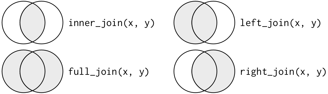
The action of combining tables through key identifiers is called “joining”. For convenience’s sake here we’ll talk about two tables X and Y, Wickham and Grolemund (2017) defines two categories of joins:

In “mutating joins”, the resulting table combines the variables from X and Y, creating a new table with variables from both X and Y, with rows that are the result of finding (different kinds of) matches between the keys of X and Y. This is the equivalent of dplyr::mutate().
In “filtering joins”, the resulting table looks in Y for entries from X, and filters the resulting table without creating or combining variables. This is the equivalent of using dplyr::filter().

I can’t recommend enough the diagrams that Hadley Wickham and Grolemund (2017) provides in R4DS–take a look at these to understand all of the variations of joins. I will not have time to over all of them here.

We will look at the most common example of each in my workflow.

7.4.2.1 mutating joins with `left_join()`

A left join looks up each unique key in X, finds the first match for that key in Y, and then adds all the columns from Y to X in the order that matches the columns in X. If there is no match for a particular key in X, the join will create an empty (NA) field. This is the most common case for joining, and it is what we were trying to accomplish with our column binding example above.

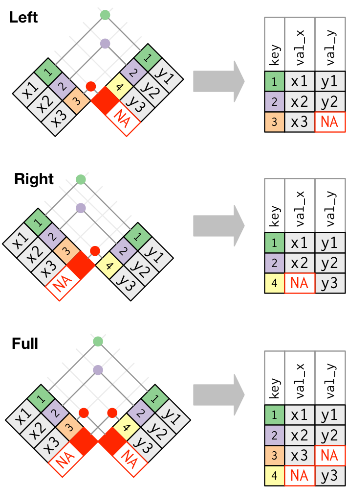
Schematic diagrams of mutating joins from Wickham and Grolemund (2017)

In tidyverse, the function for making a left join is easy to remember: left_join(). It takes as input two tables, with the first one provided being used as X (the “left”) table, and the second being “Y”. If the tables have the same named key columns, left_join() will try to join using this, but it’s usually best to explicitly provide the by = argument to left_join(), because if you have two similarly named columns that are not unique keys, this could cause errors.

# by using the pipe, tidy_cider_cata becomes X, and tidy_cider_liking becomes Y
joined_cider_cata <- tidy_cider_cata %>%
# Notice here we specify the keys, and if they are named differently we write it as <"x_key"> = <"y_key">
    left_join(tidy_cider_liking, by = c("Panelist_Name", "Sample_Name" = "cider_name"))

Notice that I used a named vector to specify the keys to join on. This might look weird, but the reason it is written as above is because both tables have subjects in the Panelist_Name column, but the names of the cider are in tidy_cider_cata$Sample_Name and tidy_cider_liking$cider_name. We are telling left_join() a vector of characters that name the columns that are keys, and in the case when they are not the same we are explicitly specifying this.

If I hadn’t done this, we would see some weird results:

# What is this using as the joining key?  What will the result be?
tidy_cider_cata %>%
  left_join(tidy_cider_liking)

## # A tibble: 52,416 × 6
##    Sample_Name Panelist_Name   cata_attribute  checked cider_name       liking
##    <chr>       <chr>           <chr>             <dbl> <chr>             <dbl>
##  1 Bold rock   Paulette Cairns FermentedApples       0 Bold rock             8
##  2 Bold rock   Paulette Cairns FermentedApples       0 Buskeys               4
##  3 Bold rock   Paulette Cairns FermentedApples       0 Blue Bee              1
##  4 Bold rock   Paulette Cairns FermentedApples       0 Potters               5
##  5 Bold rock   Paulette Cairns FermentedApples       0 Cobbler Mountain      5
##  6 Bold rock   Paulette Cairns FermentedApples       0 Big Fish              3
##  7 Bold rock   Paulette Cairns OverripeApples        0 Bold rock             8
##  8 Bold rock   Paulette Cairns OverripeApples        0 Buskeys               4
##  9 Bold rock   Paulette Cairns OverripeApples        0 Blue Bee              1
## 10 Bold rock   Paulette Cairns OverripeApples        0 Potters               5
## # … with 52,406 more rows
## # ℹ Use `print(n = ...)` to see more rows

We can check that our join worked properly by looking at that same means table we checked before. Note that this check is for this case, specifically–this does not guarantee that things have gone right in every possible situation.

# This looks right - check back to see if it matches
joined_cider_cata %>% group_by(Sample_Name) %>% summarize(mean = mean(liking))

## # A tibble: 6 × 2
##   Sample_Name       mean
##   <chr>            <dbl>
## 1 Big Fish          5.61
## 2 Blue Bee          3.95
## 3 Bold rock         6.70
## 4 Buskeys           6.05
## 5 Cobbler Mountain  4.82
## 6 Potters           4.98

What if we wanted to reverse the join, and use tidy_cider_liking as the left-side (X)? Because it is the “one” in the one-to-many relationship, we’d either have to decide on a specific CATA attribute we want to join, or rethink our resulting structure.

tidy_cider_liking %>%
  left_join(cider_cata, by = c("Panelist_Name", "cider_name" = "Sample_Name")) %>%
  select(1:8)

## # A tibble: 336 × 8
##    Panelist_Name          cider…¹ liking Ferme…² Overr…³ Fresh…⁴ Alcohol WineL…⁵
##    <chr>                  <chr>    <dbl>   <dbl>   <dbl>   <dbl>   <dbl>   <dbl>
##  1 Paulette Cairns        Bold r…      8       0       0       1       0       0
##  2 Paulette Cairns        Buskeys      4       1       0       0       1       0
##  3 Paulette Cairns        Blue B…      1       0       0       0       0       0
##  4 Paulette Cairns        Potters      5       1       0       0       0       0
##  5 Paulette Cairns        Cobble…      5       0       1       1       0       0
##  6 Paulette Cairns        Big Fi…      3       0       0       0       1       0
##  7 Renata Vieira Carneiro Bold r…      8       0       0       0       0       0
##  8 Renata Vieira Carneiro Buskeys      8       1       0       0       0       0
##  9 Renata Vieira Carneiro Blue B…      4       1       0       0       1       0
## 10 Renata Vieira Carneiro Potters      4       0       0       0       0       0
## # … with 326 more rows, and abbreviated variable names ¹cider_name,
## #   ²FermentedApples, ³OverripeApples, ⁴FreshApples, ⁵WineLike
## # ℹ Use `print(n = ...)` to see more rows

Note that we now have equivalent data structures–we could have gotten either of these by joining and then using either pivot_longer() or pivot_wider(). This is because the unique key identifiers here that we are joining on are the combination of subject and cider.

Another way to look at joins from Wickham and Grolemund (2017)

7.4.2.2 filtering joins with `anti_join()`

Filtering joins let you use a Y table as a reference for selecting rows–rather than columns–from X. In the case of anti_join(), as the name implies, this removes all rows from X that match the keys in Y.

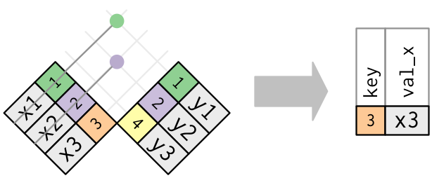
Schematic of filtering with anti-joins from Wickham and Grolemund (2017)

Let’s imagine that we had a list of panelists who had been removed from our lab for rowdy behavior. We know their results are bad because they were busy partying. Let’s create a fake list of these panelists, and then use anti_join() to take them out of our datasets.

banned_panelists <- cider_liking %>%
  slice_sample(n = 7)

tidy_cider_liking %>%
  anti_join(banned_panelists, by = "Panelist_Name")

## # A tibble: 294 × 3
##    Panelist_Name          cider_name       liking
##    <chr>                  <chr>             <dbl>
##  1 Renata Vieira Carneiro Bold rock             8
##  2 Renata Vieira Carneiro Buskeys               8
##  3 Renata Vieira Carneiro Blue Bee              4
##  4 Renata Vieira Carneiro Potters               4
##  5 Renata Vieira Carneiro Cobbler Mountain      6
##  6 Renata Vieira Carneiro Big Fish              4
##  7 Jennifer Acuff         Bold rock             4
##  8 Jennifer Acuff         Buskeys               6
##  9 Jennifer Acuff         Blue Bee              5
## 10 Jennifer Acuff         Potters               6
## # … with 284 more rows
## # ℹ Use `print(n = ...)` to see more rows

tidy_cider_cata %>%
  anti_join(banned_panelists, by = "Panelist_Name")

## # A tibble: 7,644 × 4
##    Sample_Name Panelist_Name          cata_attribute  checked
##    <chr>       <chr>                  <chr>             <dbl>
##  1 Bold rock   Renata Vieira Carneiro FermentedApples       0
##  2 Bold rock   Renata Vieira Carneiro OverripeApples        0
##  3 Bold rock   Renata Vieira Carneiro FreshApples           0
##  4 Bold rock   Renata Vieira Carneiro Alcohol               0
##  5 Bold rock   Renata Vieira Carneiro WineLike              0
##  6 Bold rock   Renata Vieira Carneiro Floral                0
##  7 Bold rock   Renata Vieira Carneiro Tart                  0
##  8 Bold rock   Renata Vieira Carneiro Candied               0
##  9 Bold rock   Renata Vieira Carneiro Fruity                1
## 10 Bold rock   Renata Vieira Carneiro Berries               0
## # … with 7,634 more rows
## # ℹ Use `print(n = ...)` to see more rows

Note that in both cases we see the number of rows go down as these rows are removed through anti_join(). We also see that we can keep a table that is separate and refer to it–this is useful if we programmatically update it (say we are always keeping a “do not serve” list) and for clarity in coding.

7.4.2.3 other joins

For a more complete documentation of other joins, I once again recommend the R4DS section or checking out ?left_join.

7.5 Writing readable and reproducible scripts

Finally, it’s a good time to revisit some principles for writing scripts and R Markdowns that will work well in the future. We’ll keep this brief and use the headers as discussion points, rather than exhaustive explorations.

7.5.1 Comments

In general, when we are coding we are very focused on the problem at hand. We’ll try a bunch of stuff, and then go with what works. But our solutions are often not clear from the code itself. Use # in order to provide comments in the code itself, explaining what each chunk or line does. Especially if you’ve written something compact and clever, like the map() functions above, it may require a lot of effort for someone else (or your future self) to interpret. Comments will help your code be useful for longer.

7.5.2 Whitespace

R is very generous about whitespace; it doesn’t enforce conventions around it. But, as we learned in week 1, writing crazily spaced code is hard to read and makes your code difficult to audit. This is even a problem with very accomplished programmers; I recommend anyone take a look at the R code in Richard McElreath (2020)’s wonderful book, which is very difficult to parse because of his arbitrary spacing and his use of uninformative variable names.

7.5.3 Use informative variable names

…speaking of which, why not help yourself and others out and use variable names that are meaningful? In older coding languages, there were limits on lengths and characters for names, so people would use conventions like “CamelCaps” and “abbrvtns”. This isn’t necessary with R, and it can make complicated commands hard to follow. If you’re coding for research, don’t do this!

7.5.4 Running from scratch

Most importantly, before you turn in assignments to me or save a project that you are done with for the moment, make sure the script/Markdown runs from scratch. Sometimes, if you’re working between the console and a script, or between multiple scripts, it’s easy to create variables or run analyses without actually writing them into your script. Or maybe you are working out of order. Restarting R, clearing all memory, and making sure it can run from the first to the last line will make sure your work survives and is reproducible.

References

McElreath, Richard. 2020. Statistical Rethinking. Second. Boca Raton: CRC Press.

Phetxumphou, Katherine, Allison N Cox, and Jacob Lahne. 2020. “Development and Characterization of a Check-All-That-Apply (CATA) Lexicon for Virginia Hard (Alcoholic) Ciders.” Journal of the American Society of Brewing Chemists, 1–10. https://doi.org/10.1080/03610470.2020.1768784.

Wickham, Hadley, and Garrett Grolemund. 2017. R for Data Science. Sebastopol: O’Reilly.

7 Advancing our wrangling

7.1 Today’s data

7.2 Review of control flow

7.2.1 Loops

7.2.1.1 for loop review

7.2.1.2 while loop review

7.2.2 Conditionals

7.3 Using vectorization in R

7.3.1 tidyverse approaches: map() family

7.3.1.1 Anonymous functions

7.3.2 Base R approaches: apply() family

7.4 Relational data

7.4.1 *bind() functions

7.4.1.1 row binding

7.4.1.2 column binding

7.4.2 *_join() functions

7.4.2.1 mutating joins with left_join()

7.4.2.2 filtering joins with anti_join()

7.4.2.3 other joins

7.5 Writing readable and reproducible scripts

7.5.1 Comments

7.5.2 Whitespace

7.5.3 Use informative variable names

7.5.4 Running from scratch

References

References

7.2.1.1 `for` loop review

7.2.1.2 `while` loop review

7.3.1 `tidyverse` approaches: `map()` family

7.3.2 Base R approaches: `apply()` family

7.4.1 `*bind()` functions

7.4.2 `*_join()` functions

7.4.2.1 mutating joins with `left_join()`

7.4.2.2 filtering joins with `anti_join()`