10 Dealing with multiple factors

10.1 Introduction

Last week, we learned the basics of the linear model: how we might try to predict a continuous outcome based on a single continuous (regression) or categorical (ANOVA) predictor. This week, we’re going to tackle the much more common situation of having multiple (even many) possible predictors for a single continuous or categorical outcome.

We’re going to switch up the order slightly and start by talking about multi-way ANOVA, which extends the basic model of ANOVA you have become somewhat familiar with to the case of multiple, categorical predictor variables. As you might guess, we are then going to talk about multiple regression, which extends regression to predicting a single, continuous outcome from multiple continuous or categorical predictors. Finally–and I am very excited and nervous to present this material–we’re going to dip our toes into one of the more modern, increasingly popular methods for predicting a single continuous or categorical outcome from multiple (many) predictors: categorization and regression tree (CART) models. These are powerful approaches that are the beginning of what we often refer to as machine learning, but we will be exploring them in their most accessible form.

10.1.1 Data example

This week, we are going to build on the berry data from last week. If you glanced at the paper, you might have seen that we didn’t just collect liking data: we collected a whole bunch of other results about each berry. In order to keep our data manageable, we are going to work only with strawberry data and Labeled Affective Magnitude (LAM) outcomes, which gives us a much smaller dataset without all of the NAs we were dealing with last week.

skim(berry_data)

Table 8.1: Data summary
Name	berry_data
Number of rows	510
Number of columns	24
_______________________
Column type frequency:
character	1
factor	5
numeric	18
________________________
Group variables	None

Variable type: character

skim_variable	n_missing	complete_rate	min	max	empty	n_unique	whitespace
berry	0	1	10	10	0	1	0

Variable type: factor

skim_variable	complete_rate	ordered	n_unique	top_counts
subject	1	FALSE	85	103: 6, 103: 6, 103: 6, 103: 6
age	1	TRUE	3	36-: 222, 21-: 144, 51-: 144
gender	1	FALSE	2	fem: 426, mal: 84
sample	1	FALSE	6	1: 85, 2: 85, 3: 85, 4: 85
percent_shopping	1	TRUE	2	75-: 366, 50-: 144

Variable type: numeric

skim_variable	complete_rate	mean	sd	p0	p25	p50	p75	p100	hist
lms_appearance	1	13.23	39.04	-92	-10.00	13	40.00	99	▂▃▇▇▂
lms_overall	1	15.29	41.98	-100	-10.00	13	51.00	100	▁▃▇▇▃
lms_taste	1	10.65	43.99	-100	-21.75	12	42.75	100	▂▅▇▇▃
lms_texture	1	21.13	39.81	-99	-7.75	27	54.00	100	▁▂▆▇▃
lms_aroma	1	19.47	33.39	-78	-1.00	12	45.75	99	▁▁▇▅▂
cata_taste_floral	1	0.15	0.36	0	0.00	0	0.00	1	▇▁▁▁▂
cata_taste_berry	1	0.46	0.50	0	0.00	0	1.00	1	▇▁▁▁▇
cata_taste_grassy	1	0.31	0.46	0	0.00	0	1.00	1	▇▁▁▁▃
cata_taste_fermented	1	0.14	0.35	0	0.00	0	0.00	1	▇▁▁▁▁
cata_taste_fruity	1	0.42	0.49	0	0.00	0	1.00	1	▇▁▁▁▆
cata_taste_citrus	1	0.18	0.38	0	0.00	0	0.00	1	▇▁▁▁▂
cata_taste_earthy	1	0.26	0.44	0	0.00	0	1.00	1	▇▁▁▁▃
cata_taste_none	1	0.06	0.24	0	0.00	0	0.00	1	▇▁▁▁▁
cata_taste_peachy	1	0.08	0.27	0	0.00	0	0.00	1	▇▁▁▁▁
cata_taste_caramel	1	0.03	0.17	0	0.00	0	0.00	1	▇▁▁▁▁
cata_taste_grapey	1	0.11	0.32	0	0.00	0	0.00	1	▇▁▁▁▁
cata_taste_melon	1	0.10	0.29	0	0.00	0	0.00	1	▇▁▁▁▁
cata_taste_cherry	1	0.11	0.32	0	0.00	0	0.00	1	▇▁▁▁▁

In this dataset, we now have not only lms_overall, but several other lms_* variables, which represent LAM liking for different modalities: taste, texture, etc. We also have a large number of cata_* variables, which represent “Check All That Apply” (CATA) questions asking subjects to indicate the presence or absence of a particular flavor. As before, our goal will be to understand overall liking, represented by the familiar lms_overall, but we will be using a new set of tools to do so.

10.2 Multi-way ANOVA

When we first examined this dataset via ANOVA, we investigated the effect of the categorical predictor berry type on us_overall (recall this was our unstructured line-scale outcome). This week we will be mostly focusing on lms_overall as the outcome variable, and we’ve limited ourselves to berry == "strawberry" because we wanted a consistent set of “CATA” attributes (and less missing data). But we have added a lot of other predictor variables–both categorical (factor) and continuous (numeric) predictors.

To motivate the idea of multi-way ANOVA, let’s think about how we might see differences in overall scale use by subject. This is a common issue in any kind of human-subjects research:

berry_data %>%
  ggplot(aes(x = subject, y = lms_overall, color = sample)) + 
  geom_point(alpha = 0.5) +
  geom_hline(yintercept = 0, color = "black", linetype = "dashed") +
  theme_bw() +
  scale_color_viridis_d() + 
  theme(axis.text.x = element_text(angle = 90, size = 6))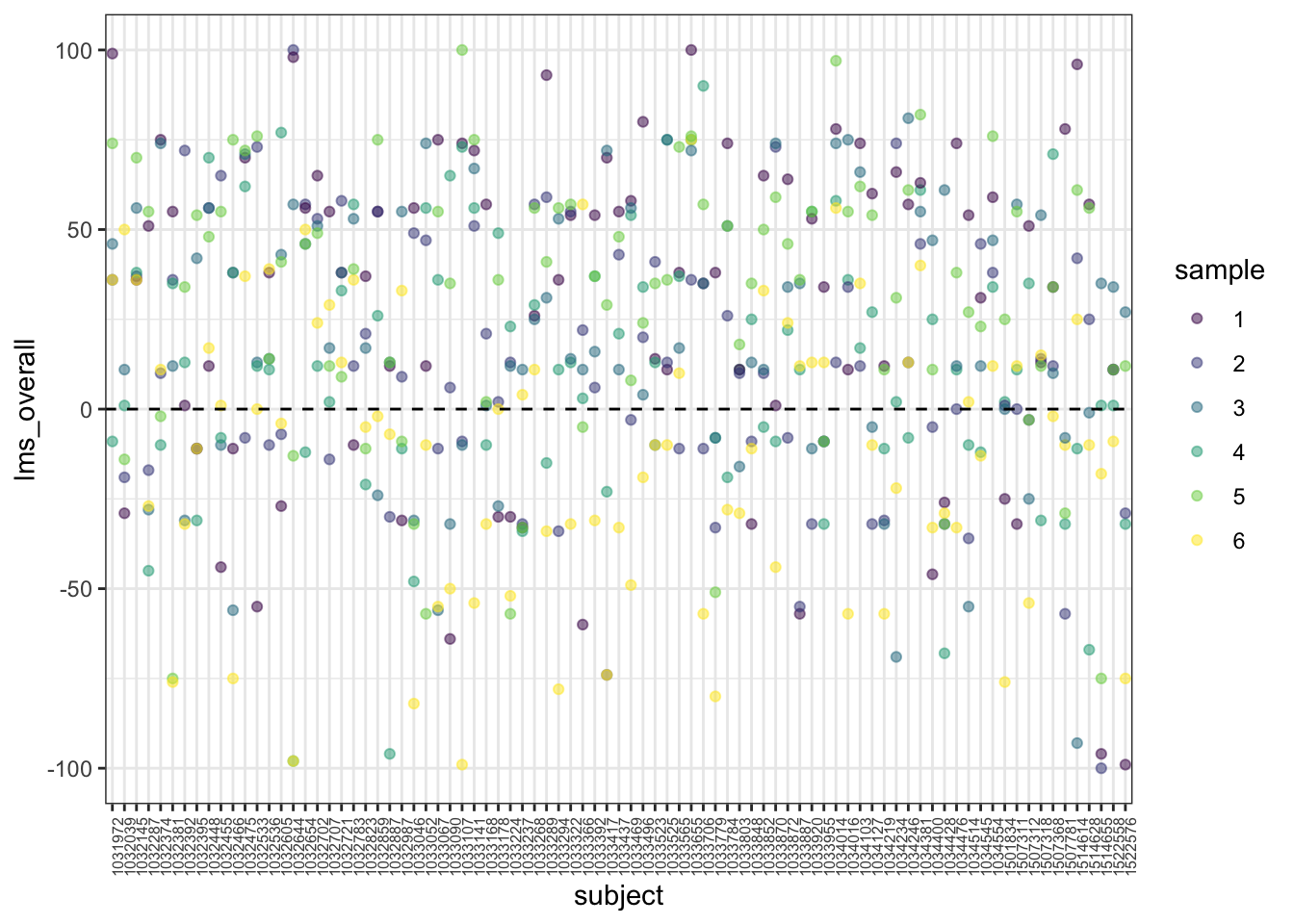

We can see that some subjects tend to use the upper part of the scale, and that while we see subjects are less likely to use the negative side of the scale (“endpoint avoidance”), some subjects are more likely to use the full scale than others. This indicates that the fact we have repeated measurements from each subject may introduce some nuisance patterns to our data.

Now, let’s imagine we want to predict lms_overall based on how much shopping each subject does for their household. This is slightly arbitrary, but we could imagine our thought process is: “Well, those who buy a lot of strawberries might have stronger opinions about strawberry flavor than those who do less.” We learned how to set up a 1-way ANOVA last week:

# How do we set up a 1-way ANOVA for lms_overall dependent on percent_shopping

We can see that overall the effect is not significant (unsurprisingly), but perhaps the effect is obscured by the variation we noted in individual scale use by subject. We can use a multiway ANOVA to investigate this possibility:

berry_data %>%
  aov(lms_overall ~ percent_shopping * subject, data = .) %>%
  summary()

##                   Df Sum Sq Mean Sq F value   Pr(>F)    
## percent_shopping   1    142   142.2   0.090 0.763706    
## subject           83 229247  2762.0   1.758 0.000181 ***
## Residuals        425 667758  1571.2                     
## ---
## Signif. codes:  0 '***' 0.001 '**' 0.01 '*' 0.05 '.' 0.1 ' ' 1

Hmm, well unsurprisingly that’s nothing either, although you can see that the effect-size estimate (F-statistic) for percent_shopping increased very slightly.

We use the same function, aov(), to build multi-way ANOVA models, and the only difference is that we will add a new set of tools to our formula interface:

+ adds a main effect for a term to our formula
<variable 1> * <variable 2> interacts the two (or more) variables as well as adding all lower-level interactions and main effects
<variable 1> : <variable 2> adds only the interaction term between the two (or more) variables

The type of model we just fit is often called a “blocked” design: our subjects are formally declared to be experimental “blocks” (units), and we accounted for the effect of differences in these blocks by including them in our model. This is why our estimate for the effect of percent_shopping increased slightly. This is the simplest example of a mixed-effects model, which are the subject of extensive research and writing. For more information on different kinds of ANOVA models, I highly recommend Statistical methods for psychology by David Howell (2010). While he does not write the textbook using R, his personal webpage (charmingly antiquated looking) has a huge wealth of information and R scripts for a number of statistical topics, including resampling approaches to ANOVA.

You might note that we asked for the interaction (percent_shopping * subject) but we got no interaction effect in our model output. What gives? Well, subject is entirely nested within percent_shopping–if we know the subject variable we already know what percent_shopping they are responsible for. Let’s take a look at a model in which we predict lms_overall from some variables that do not have this relationship:

berry_data %>%
  aov(lms_overall ~ percent_shopping * age * sample, data = .) %>%
  summary()

##                              Df Sum Sq Mean Sq F value   Pr(>F)    
## percent_shopping              1    142     142   0.090   0.7646    
## age                           2   8369    4184   2.643   0.0722 .  
## sample                        5 101078   20216  12.766 1.17e-11 ***
## percent_shopping:age          2   2959    1479   0.934   0.3936    
## percent_shopping:sample       5   7195    1439   0.909   0.4750    
## age:sample                   10  12143    1214   0.767   0.6609    
## percent_shopping:age:sample  10  14675    1467   0.927   0.5081    
## Residuals                   474 750586    1584                     
## ---
## Signif. codes:  0 '***' 0.001 '**' 0.01 '*' 0.05 '.' 0.1 ' ' 1

Here we see a number of interactions, none of them “signficant”. Again, this makes sense–honestly, it’s unclear why age, gender, or percent_shopping would really predict overall liking for strawberry varieties. But we do see the estimated interaction effects, like percent_shopping:age.

Let’s try running one more multi-way ANOVA for variables we might actually expect to predict lms_overall: some of the CATA variables. These are binary variables that indicate the presence or absence of a particular sensory attribute. There are a lot of them. We are going to just pick a couple and see if they predict overall liking:

berry_data %>%
  aov(lms_overall ~ cata_taste_berry * cata_taste_fruity * cata_taste_fermented * sample, 
      data = .) %>%
  anova() %>% # the anova() function returns a data.frame, unlike summary()
  as_tibble(rownames = "effect") # purely for printing kind of nicely

## # A tibble: 16 × 6
##    effect                                   Df Sum S…¹ Mean …² F val…³  `Pr(>F)`
##    <chr>                                 <int>   <dbl>   <dbl>   <dbl>     <dbl>
##  1 cata_taste_berry                          1  2.98e5  2.98e5 300.     2.86e-52
##  2 cata_taste_fruity                         1  4.74e4  4.74e4  47.7    1.61e-11
##  3 cata_taste_fermented                      1  3.05e4  3.05e4  30.7    5.15e- 8
##  4 sample                                    5  3.07e4  6.14e3   6.18   1.47e- 5
##  5 cata_taste_berry:cata_taste_fruity        1  9.93e1  9.93e1   0.100  7.52e- 1
##  6 cata_taste_berry:cata_taste_fermented     1  2.57e3  2.57e3   2.58   1.09e- 1
##  7 cata_taste_fruity:cata_taste_ferment…     1  2.13e3  2.13e3   2.15   1.43e- 1
##  8 cata_taste_berry:sample                   5  4.26e3  8.52e2   0.857  5.10e- 1
##  9 cata_taste_fruity:sample                  5  4.43e3  8.86e2   0.892  4.86e- 1
## 10 cata_taste_fermented:sample               5  3.60e3  7.20e2   0.725  6.05e- 1
## 11 cata_taste_berry:cata_taste_fruity:c…     1  1.63e2  1.63e2   0.164  6.86e- 1
## 12 cata_taste_berry:cata_taste_fruity:s…     5  1.05e3  2.11e2   0.212  9.57e- 1
## 13 cata_taste_berry:cata_taste_fermente…     5  1.64e3  3.29e2   0.331  8.94e- 1
## 14 cata_taste_fruity:cata_taste_ferment…     4  1.12e3  2.81e2   0.283  8.89e- 1
## 15 cata_taste_berry:cata_taste_fruity:c…     3  6.89e3  2.30e3   2.31   7.54e- 2
## 16 Residuals                               465  4.62e5  9.94e2  NA     NA       
## # … with abbreviated variable names ¹`Sum Sq`, ²`Mean Sq`, ³`F value`

Here we can see a lot of things (probably too many things, as we’ll get to in a moment). But I want to point out several aspects of this model that are of interest to us:

The main effects of the CATA variables are all significant, as is the sample variable: the data tell us that the different strawberry samples are liked differently, and that the presence or absence of these 3 CATA variables matters as well.
None of the interactions are very important. This means that different CATA effects, for example, don’t matter differently for overall liking for different samples.
Because we requested interactions among 4 variables, we get estimates of interactions up to 4-way interactions. This is a lot of information, and probably an “overfit” model.

However, we picked 3 CATA variables at random. There are 13 of these actually collected. If even 4-way interactions are probably overfit, how can we possibly pick which of these to include in our model? We will learn about a data-driven approach to this called a “Partition Tree” later today, but for now let’s look at a classic approach: stepwise regression/ANOVA.

10.2.1 Stepwise model fitting

Imagine we have a large number of predictor variables, and part of our analysis needs are deciding which to include in a model. This is a common situation, as it corresponds to the general research question: “Which treatments actually matter?”

We can approach this question by letting our data drive the analysis. We know about \(R^2\), which is an estimate of how well our model fits the data. There are many other fit criteria. What if we just add variables to our model if they make it fit the data better? This is a reasonable (although very risky, it turns out!) approach that is quite common. This is often called “stepwise model selection” or “fitting”.

# We first subset our data for ease of use to just the variables we will consider
berry_cata <- berry_data %>% select(lms_overall, sample, contains("cata"))

# Then we fit a model with no variables
intercept_only <- aov(lms_overall ~ 1, data = berry_cata)

# And we fit a model with ALL possible variables
all <- aov(lms_overall ~ .^2, data = berry_cata)

# Finally, we tell R to "step" between the no-variable model and the model with
# all the variables.  At each step, R will consider all possible variables to
# add to or subtract from the model, based on which one will most decrease a
# fit criterion called the AIC (don't worry about it right now).  This will 
# be repeated until the model can no longer be improved, at which point we have
# a final, data-driven model
stepwise <- step(intercept_only, direction = "both", scope = formula(all), trace = 0)
anova(stepwise) %>% as_tibble(rownames = "effect")

## # A tibble: 18 × 6
##    effect                                   Df Sum S…¹ Mean …² F val…³  `Pr(>F)`
##    <chr>                                 <int>   <dbl>   <dbl>   <dbl>     <dbl>
##  1 cata_taste_berry                          1 298464. 298464. 339.     9.44e-58
##  2 cata_taste_fruity                         1  47443.  47443.  53.9    9.15e-13
##  3 cata_taste_fermented                      1  30470.  30470.  34.6    7.59e- 9
##  4 sample                                    5  30699.   6140.   6.97   2.66e- 6
##  5 cata_taste_floral                         1  11900.  11900.  13.5    2.64e- 4
##  6 cata_taste_caramel                        1   8830.   8830.  10.0    1.64e- 3
##  7 cata_taste_earthy                         1   2848.   2848.   3.23   7.28e- 2
##  8 cata_taste_melon                          1   2803.   2803.   3.18   7.50e- 2
##  9 cata_taste_none                           1    694.    694.   0.788  3.75e- 1
## 10 cata_taste_berry:cata_taste_floral        1   4671.   4671.   5.30   2.17e- 2
## 11 cata_taste_berry:cata_taste_caramel       1   3576.   3576.   4.06   4.45e- 2
## 12 sample:cata_taste_earthy                  5  11938.   2388.   2.71   1.98e- 2
## 13 cata_taste_fermented:cata_taste_melon     1   5446.   5446.   6.18   1.32e- 2
## 14 cata_taste_berry:cata_taste_earthy        1   3069.   3069.   3.48   6.25e- 2
## 15 cata_taste_berry:cata_taste_fermented     1   3902.   3902.   4.43   3.58e- 2
## 16 cata_taste_fruity:cata_taste_none         1   2309.   2309.   2.62   1.06e- 1
## 17 cata_taste_floral:cata_taste_melon        1   1779.   1779.   2.02   1.56e- 1
## 18 Residuals                               484 426306.    881.  NA     NA       
## # … with abbreviated variable names ¹`Sum Sq`, ²`Mean Sq`, ³`F value`

# We can also see the actual effect on lms_overall of the selected variables
stepwise$coefficients %>% as_tibble(rownames = "effect")

## # A tibble: 26 × 2
##    effect                 value
##    <chr>                  <dbl>
##  1 (Intercept)           -3.02 
##  2 cata_taste_berry      38.5  
##  3 cata_taste_fruity     17.3  
##  4 cata_taste_fermented -28.0  
##  5 sample2              -10.7  
##  6 sample3               -1.70 
##  7 sample4               -7.15 
##  8 sample5                0.634
##  9 sample6              -24.3  
## 10 cata_taste_floral     23.6  
## # … with 16 more rows
## # ℹ Use `print(n = ...)` to see more rows

This kind of step-wise approach is very common, but it is also potentially problematic, as it finds a solution that fits the data, not the question. Whether this model will predict future outcomes is unclear. It is always a good idea when using these approaches to test the new model on unseen data, or to treat these approaches as exploratory rather than explanatory approaches: they are good for generating future, testable hypotheses, rather than giving a final answer or prediction.

Therefore, in our example, we might generate a hypothesis for further testing: “It is most important for strawberries to have ‘berry’, ‘fruity’, and not ‘fermented’ tastes for overall consumer acceptability.” We can then test this by obtaining berries known to have those qualities and testing whether, for example, more “berry”-like strawberries are indeed better liked.

10.2.2 Plotting interaction effects

We really don’t have much in the way of interaction effects in our ANOVA models, but let’s look at how we might visualize those effects–this is one of the most effective ways to both understand and communicate about interacting variables in multi-way models.

# First, we'll set up a summary table for our data: we want the mean lms_overall 
# for each berry sample for when cata_taste_fermented == 0 and == 1
example_interaction_data <- berry_data %>%
  group_by(sample, cata_taste_fermented) %>%
  summarize(mean_liking = mean(lms_overall),
            se_liking = sd(lms_overall)/sqrt(n()))
example_interaction_data

## # A tibble: 12 × 4
## # Groups:   sample [6]
##    sample cata_taste_fermented mean_liking se_liking
##    <fct>                 <dbl>       <dbl>     <dbl>
##  1 1                         0       36.4       4.88
##  2 1                         1      -17.5      14.1 
##  3 2                         0       17.6       3.77
##  4 2                         1      -26        13.8 
##  5 3                         0       20.7       4.30
##  6 3                         1       20.8      15.5 
##  7 4                         0       14.9       4.23
##  8 4                         1      -12.1      14.7 
##  9 5                         0       37.2       3.74
## 10 5                         1       -7.46     13.6 
## 11 6                         0       -5.69      4.37
## 12 6                         1      -35.7      10.4

# Now we can use this to draw a plot illustrating the INTERACTION of sample and 
# cata_taste_fermented on lms_overall
p <- example_interaction_data %>%
  ggplot(aes(x = cata_taste_fermented, y = mean_liking, color = sample)) + 
  geom_point() + 
  geom_errorbar(aes(ymin = mean_liking - 2 * se_liking, 
                    ymax = mean_liking + 2 * se_liking),
                linetype = "dashed", width = 0.1) +
  geom_line() + 
  theme_classic() + 
  scale_color_viridis_d()

p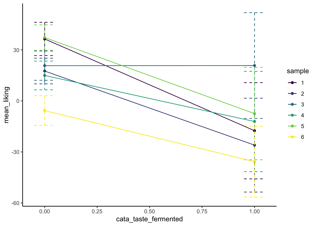

We can see that there may in fact be some kind of interactive effect, in that while overall it seems like presence of a “fermented” flavor decreases liking for most samples, it doesn’t have much of an effect on Sample 3. But we don’t see this as an overall effect in our model, and our uncertainty (error) bars indicate why this might be: it seems like there is such high variability in that sample’s lms_overall ratings that we can’t say for sure whether that mean estimate is very reliable–I would go so far as to say we’d want do some further exploration of that sample itself in order to understand why it is so much more variable than the other samples.

# This is an interactive plot from the plotly package, which you may enjoy 
# fooling around with as you move forward.  It makes seeing plot elements a
# little easier in complex plots.

# It is possible to render ggplots interactive in one step
# (mostly) by saving them and using the ggplotly() function.
plotly::ggplotly(p)

10.3 Multiple regression

So far we have focused our thinking on multiple, categorical predictors: variables that can take one of a set of discrete values. This is advantageous for learning about interactions, because it is much easier to visualize the interaction of categorical variables through interactions like those above.

But what if we have several continuous predictors? Just as simple regression and ANOVA are analogues of each other, multiple regression is the equivalent of multi-way ANOVA when one or more of the predictors is continuous instead of categorical (when we have a mix of continuous and categorical variables we tend to deal with them through either multiple regression or with something called ANCOVA: Analysis of Co-Variance).

Multiple regression involves predicting the value of an outcome from many continuous or categorical predictors. Multiple regression is also a topic that deserves (and is taught as) a course-length topic in its own right (see for example STAT 6634). I will be barely scratching the surface of multiple regression here–as always, I am going to attempt to show you how to implement a method in R.

We can frame our objective in multiple regression as predicting the value of a single outcome \(y\) from a set of predictors \(x_1, x_2, ..., x_n\).

\(\hat{y}_i = \beta_1 * x_{1i} + \beta_2 * x_{2i} + ... + \beta_n * x_{ni} + \alpha\)

The tasks in multiple regression are:

To develop a model that predicts \(y\)
To identify variables \(x_1, x_2, ...\) etc that are actually important in predicting \(y\)

The first task is usually evaluated in the same way as we did in simple regression–by investigating goodness-of-fit statistics like \(R^2\). This is often interpreted as overall quality of the model.

The second task is often considered more important in research applications: we want to understand which \(x\)-variables significantly predict \(y\). We usually assess this by investigating statistical significance of the \(\beta\)-coefficients for each predictor.

Finally, a third and important task in multiple regression is identifying interacting predictor variables. In my usual, imprecise interpretation, an interactive effect can be stated as “the effect of \(x_1\) is different at different values of \(x_2\)”–this means that we have a multiplicative effect in our model.

The model given above omits interactive terms, which would look like:

\(\hat{y}_i = \beta_1 * x_{1i} + \beta_2 * x_{2i} + ... + \beta_n * x_{ni} + \beta_{1*2} * x_{1i} * x_{2i} + ... + \alpha\)

You can see why I left them out!

10.3.1 Fitting a multiple regression to our model

It’s been long enough–let’s review what our dataset looks like:

berry_data %>%
  glimpse

## Rows: 510
## Columns: 24
## $ subject              <fct> 1033784, 1033784, 1033784, 1033784, 1033784, 1033…
## $ age                  <ord> 51-65, 51-65, 51-65, 51-65, 51-65, 51-65, 51-65, …
## $ gender               <fct> female, female, female, female, female, female, f…
## $ berry                <chr> "strawberry", "strawberry", "strawberry", "strawb…
## $ sample               <fct> 4, 1, 2, 6, 3, 5, 4, 1, 2, 6, 3, 5, 4, 1, 2, 6, 3…
## $ percent_shopping     <ord> 75-100%, 75-100%, 75-100%, 75-100%, 75-100%, 75-1…
## $ lms_appearance       <dbl> 9, 68, 11, 47, 71, 68, 73, 13, -11, -13, 75, 37, …
## $ lms_overall          <dbl> -19, 74, 26, -28, 51, 51, 57, -10, 12, 36, 53, 39…
## $ lms_taste            <dbl> -3, 77, 27, -28, 51, 48, 39, -10, 14, 25, 57, 34,…
## $ lms_texture          <dbl> 20, 72, 27, 30, 68, 63, 72, 37, 53, 36, 77, 39, 1…
## $ lms_aroma            <dbl> -1, 81, 76, 57, 72, 21, -29, 11, -1, 1, 58, -11, …
## $ cata_taste_floral    <dbl> 0, 1, 0, 0, 1, 0, 0, 0, 0, 0, 0, 0, 0, 0, 0, 1, 0…
## $ cata_taste_berry     <dbl> 0, 1, 1, 0, 1, 1, 0, 0, 0, 0, 0, 0, 1, 1, 1, 0, 0…
## $ cata_taste_grassy    <dbl> 0, 0, 0, 1, 0, 0, 0, 0, 0, 0, 0, 0, 0, 0, 0, 1, 1…
## $ cata_taste_fermented <dbl> 0, 0, 0, 0, 0, 0, 0, 0, 0, 0, 0, 0, 0, 0, 0, 0, 0…
## $ cata_taste_fruity    <dbl> 0, 1, 1, 0, 1, 1, 0, 1, 0, 0, 1, 0, 0, 1, 1, 0, 0…
## $ cata_taste_citrus    <dbl> 0, 0, 0, 0, 0, 0, 0, 0, 0, 0, 0, 0, 0, 0, 0, 0, 0…
## $ cata_taste_earthy    <dbl> 0, 0, 0, 1, 0, 0, 0, 0, 0, 0, 0, 0, 0, 0, 0, 1, 1…
## $ cata_taste_none      <dbl> 1, 0, 0, 0, 0, 0, 1, 0, 1, 1, 0, 1, 0, 0, 0, 0, 0…
## $ cata_taste_peachy    <dbl> 0, 0, 0, 0, 0, 0, 0, 0, 0, 0, 0, 0, 1, 0, 0, 0, 0…
## $ cata_taste_caramel   <dbl> 0, 0, 0, 0, 0, 0, 0, 0, 0, 0, 0, 0, 0, 0, 0, 0, 0…
## $ cata_taste_grapey    <dbl> 0, 0, 0, 0, 0, 0, 0, 0, 0, 0, 0, 0, 0, 0, 0, 0, 0…
## $ cata_taste_melon     <dbl> 0, 0, 0, 0, 0, 0, 0, 0, 0, 0, 0, 0, 0, 0, 0, 0, 0…
## $ cata_taste_cherry    <dbl> 0, 0, 0, 0, 0, 0, 0, 0, 0, 0, 0, 0, 1, 1, 1, 0, 0…

While we have no real reason to do so, let’s build a model that predicts lms_overall from lms_appearance, lms_taste, lms_aroma, and lms_texture. We can frame the research question as: “In this dataset, can we understand overall liking as an interaction of multiple modalities?”

So we would write the model we asked for in words above as: lms_overall ~ lms_taste + lms_appearance + lms_aroma + lms_texture (notice we are not adding interactions yet).

berry_mlm <- berry_data %>%
  lm(lms_overall ~ lms_taste + lms_appearance + lms_aroma + lms_texture, data = .)

summary(berry_mlm)

## 
## Call:
## lm(formula = lms_overall ~ lms_taste + lms_appearance + lms_aroma + 
##     lms_texture, data = .)
## 
## Residuals:
##     Min      1Q  Median      3Q     Max 
## -75.936  -8.169  -0.751   8.788  88.033 
## 
## Coefficients:
##                Estimate Std. Error t value Pr(>|t|)    
## (Intercept)    3.153003   0.883068   3.571  0.00039 ***
## lms_taste      0.769195   0.022335  34.439  < 2e-16 ***
## lms_appearance 0.087427   0.021291   4.106 4.69e-05 ***
## lms_aroma      0.008425   0.024036   0.350  0.72612    
## lms_texture    0.124233   0.023159   5.364 1.24e-07 ***
## ---
## Signif. codes:  0 '***' 0.001 '**' 0.01 '*' 0.05 '.' 0.1 ' ' 1
## 
## Residual standard error: 15.66 on 505 degrees of freedom
## Multiple R-squared:  0.8619, Adjusted R-squared:  0.8608 
## F-statistic:   788 on 4 and 505 DF,  p-value: < 2.2e-16

This model explores the relationships we can visualize in various ways shown below:

library(ggforce)
berry_data %>%
  ggplot(aes(x = .panel_x, y = .panel_y)) +
  geom_point(alpha = 0.1) +
  geom_smooth(method = lm, color = "red") +
  geom_density_2d(color = "black") +
  geom_autodensity() +
  facet_matrix(rows = vars(contains("lms")), 
               cols = vars(contains("lms")), 
               layer.lower = 3, 
               layer.upper = c(1, 2), 
               layer.diag = 4) +
  theme_classic()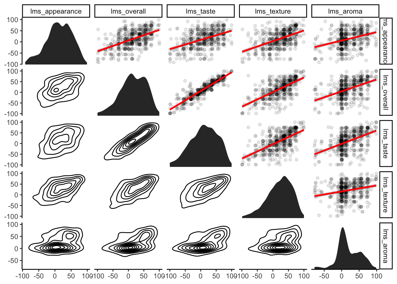

Just as in simple regression, we can use accessor functions to get coefficients, predicted values, etc.

coefficients(berry_mlm) %>% as_tibble(rownames = "effect")

## # A tibble: 5 × 2
##   effect           value
##   <chr>            <dbl>
## 1 (Intercept)    3.15   
## 2 lms_taste      0.769  
## 3 lms_appearance 0.0874 
## 4 lms_aroma      0.00842
## 5 lms_texture    0.124

# just looking at the first few predictions
head(predict(berry_mlm))

##          1          2          3          4          5          6 
##   4.108488  77.953222  28.877523 -10.068231  57.643668  54.022987

# the actual values of lms_overall
berry_data %>% head() %>% select(contains("lms")) %>% relocate(lms_overall)

## # A tibble: 6 × 5
##   lms_overall lms_appearance lms_taste lms_texture lms_aroma
##         <dbl>          <dbl>     <dbl>       <dbl>     <dbl>
## 1         -19              9        -3          20        -1
## 2          74             68        77          72        81
## 3          26             11        27          27        76
## 4         -28             47       -28          30        57
## 5          51             71        51          68        72
## 6          51             68        48          63        21

Now, we will take a look at what happens when we allow interactions in the model:

berry_mlm_interactions <- berry_data %>%
  lm(lms_overall ~ lms_taste * lms_appearance * lms_aroma * lms_texture, data = .)
anova(berry_mlm_interactions) %>% as_tibble(rownames = "effect")

## # A tibble: 16 × 6
##    effect                                 Df Sum S…¹ Mean …² F valu…³   `Pr(>F)`
##    <chr>                               <int>   <dbl>   <dbl>    <dbl>      <dbl>
##  1 lms_taste                               1  7.57e5  7.57e5  3.13e+3  5.82e-216
##  2 lms_appearance                          1  8.96e3  8.96e3  3.71e+1  2.30e-  9
##  3 lms_aroma                               1  2.42e1  2.42e1  1.00e-1  7.52e-  1
##  4 lms_texture                             1  7.06e3  7.06e3  2.92e+1  1.02e-  7
##  5 lms_taste:lms_appearance                1  7.21e1  7.21e1  2.98e-1  5.85e-  1
##  6 lms_taste:lms_aroma                     1  3.85e2  3.85e2  1.59e+0  2.07e-  1
##  7 lms_appearance:lms_aroma                1  6.57e2  6.57e2  2.72e+0  9.99e-  2
##  8 lms_taste:lms_texture                   1  2.39e2  2.39e2  9.89e-1  3.20e-  1
##  9 lms_appearance:lms_texture              1  7.95e0  7.95e0  3.29e-2  8.56e-  1
## 10 lms_aroma:lms_texture                   1  4.04e2  4.04e2  1.67e+0  1.97e-  1
## 11 lms_taste:lms_appearance:lms_aroma      1  5.38e2  5.38e2  2.23e+0  1.36e-  1
## 12 lms_taste:lms_appearance:lms_textu…     1  4.01e2  4.01e2  1.66e+0  1.99e-  1
## 13 lms_taste:lms_aroma:lms_texture         1  9.52e1  9.52e1  3.94e-1  5.31e-  1
## 14 lms_appearance:lms_aroma:lms_textu…     1  1.09e3  1.09e3  4.49e+0  3.46e-  2
## 15 lms_taste:lms_appearance:lms_aroma…     1  5.69e2  5.69e2  2.35e+0  1.26e-  1
## 16 Residuals                             494  1.19e5  2.42e2 NA       NA        
## # … with abbreviated variable names ¹`Sum Sq`, ²`Mean Sq`, ³`F value`

We have some significant higher-order interactions, but again we are ending up estimating a lot of new effects to gain very little in predictive power. We can compare the \(R^2\) for both models:

map(list(berry_mlm, berry_mlm_interactions), ~summary(.) %>% .$r.squared)

## [[1]]
## [1] 0.8619019
## 
## [[2]]
## [1] 0.8668665

We are adding a lot of “cruft” to our models without getting much in return.

10.3.2 A second example of stepwise model fitting

We can use a stepwise model fitting approach on regression just as easily as we can on ANOVA. To do so, we will follow the same steps:

Set up a “null” model that just estimates the mean of the outcome variable (lms_overall)
Set up a “full” model that includes all possible predictors for the outcome variable
Use the step() function to fit successive models until the best fit to the data is achieved

# Trim our data for convenience
berry_lms <- select(berry_data, contains('lms'))

# Set up our null model
null_model <- lm(lms_overall ~ 1, data = berry_lms)
# Set up the full model, including all possible-level interactions
full_model <- lm(lms_overall ~ .^4, data = berry_lms)
# Use step() to try all possible models
selected_model <- step(null_model, scope = formula(full_model), direction = "both", trace = 0)
summary(selected_model)

## 
## Call:
## lm(formula = lms_overall ~ lms_taste + lms_texture + lms_appearance, 
##     data = berry_lms)
## 
## Residuals:
##     Min      1Q  Median      3Q     Max 
## -75.461  -8.219  -0.825   8.963  87.996 
## 
## Coefficients:
##                Estimate Std. Error t value Pr(>|t|)    
## (Intercept)     3.28919    0.79231   4.151 3.88e-05 ***
## lms_taste       0.77229    0.02050  37.682  < 2e-16 ***
## lms_texture     0.12323    0.02296   5.367 1.22e-07 ***
## lms_appearance  0.08864    0.02099   4.223 2.86e-05 ***
## ---
## Signif. codes:  0 '***' 0.001 '**' 0.01 '*' 0.05 '.' 0.1 ' ' 1
## 
## Residual standard error: 15.65 on 506 degrees of freedom
## Multiple R-squared:  0.8619, Adjusted R-squared:  0.861 
## F-statistic:  1052 on 3 and 506 DF,  p-value: < 2.2e-16

selected_model$coefficients %>% as_tibble(rownames = "effect")

## # A tibble: 4 × 2
##   effect          value
##   <chr>           <dbl>
## 1 (Intercept)    3.29  
## 2 lms_taste      0.772 
## 3 lms_texture    0.123 
## 4 lms_appearance 0.0886

In this case the model selection process dismisses all the higher-level interactions, as well as the main effect of lms_aroma.

10.3.3 Combining continuous and categorical data

In berry_data we have both categorical and continuous predictors. Wouldn’t it be nice if we could combine them? In particular, we know that sample is an important variable, as different samples are definitely differently liked. Let’s see what happens when we include this in our multiple linear regression:

berry_mlm_cat <- berry_data %>%
# We will restrict our interactions to "2nd-order" (2-element) interactions
# Because we think 3rd- and 4th-order are unlikely to be important and they are 
# A huge mess in the output
  lm(lms_overall ~ (sample + lms_appearance + lms_taste + lms_texture + lms_aroma)^2, 
     data = .)
anova(berry_mlm_cat) %>% as_tibble(rownames = "effect")

## # A tibble: 16 × 6
##    effect                        Df   `Sum Sq`  `Mean Sq`  `F value`   `Pr(>F)`
##    <chr>                      <int>      <dbl>      <dbl>      <dbl>      <dbl>
##  1 sample                         5 101078.     20216.      84.3      2.83e- 63
##  2 lms_appearance                 1 194144.    194144.     810.       1.25e-104
##  3 lms_taste                      1 472036.    472036.    1969.       6.58e-171
##  4 lms_texture                    1   7214.      7214.      30.1      6.70e-  8
##  5 lms_aroma                      1      4.24       4.24     0.0177   8.94e-  1
##  6 sample:lms_appearance          5    852.       170.       0.711    6.15e-  1
##  7 sample:lms_taste               5   1504.       301.       1.26     2.82e-  1
##  8 sample:lms_texture             5   1681.       336.       1.40     2.22e-  1
##  9 sample:lms_aroma               5   4280.       856.       3.57     3.52e-  3
## 10 lms_appearance:lms_taste       1      2.19       2.19     0.00912  9.24e-  1
## 11 lms_appearance:lms_texture     1      0.549      0.549    0.00229  9.62e-  1
## 12 lms_appearance:lms_aroma       1    291.       291.       1.21     2.71e-  1
## 13 lms_taste:lms_texture          1     20.6       20.6      0.0858   7.70e-  1
## 14 lms_taste:lms_aroma            1    412.       412.       1.72     1.91e-  1
## 15 lms_texture:lms_aroma          1     11.7       11.7      0.0489   8.25e-  1
## 16 Residuals                    474 113615.       240.      NA       NA

coefficients(berry_mlm_cat) %>% as_tibble(rownames = "effect")

## # A tibble: 36 × 2
##    effect           value
##    <chr>            <dbl>
##  1 (Intercept)     2.86  
##  2 sample2         3.02  
##  3 sample3         1.16  
##  4 sample4        -3.95  
##  5 sample5         2.00  
##  6 sample6        -2.12  
##  7 lms_appearance  0.209 
##  8 lms_taste       0.724 
##  9 lms_texture     0.0668
## 10 lms_aroma       0.0975
## # … with 26 more rows
## # ℹ Use `print(n = ...)` to see more rows

Whoa, what just happened? Well, sample is a categorical variable with 6 levels, and when we enter it into a regression the most conventional way to deal with that data is to create a set of \(6 - 1 = 5\) “dummy” variables , and which take on a value of 1 whenever the sample is equal to that level, and 0 otherwise. That means that each adds some constant to the mean based on the estimated difference from that sample.

This is where the difference between the summary() and anova() function becomes important. If we look at the summary table for our new model with both categorical and continuous variables we see something awful:

summary(berry_mlm_cat)

## 
## Call:
## lm(formula = lms_overall ~ (sample + lms_appearance + lms_taste + 
##     lms_texture + lms_aroma)^2, data = .)
## 
## Residuals:
##     Min      1Q  Median      3Q     Max 
## -59.378  -7.651  -0.844   8.240  85.050 
## 
## Coefficients:
##                              Estimate Std. Error t value Pr(>|t|)    
## (Intercept)                 2.861e+00  2.908e+00   0.984  0.32572    
## sample2                     3.017e+00  3.540e+00   0.852  0.39453    
## sample3                     1.162e+00  3.939e+00   0.295  0.76808    
## sample4                    -3.946e+00  3.656e+00  -1.079  0.28101    
## sample5                     2.005e+00  4.209e+00   0.476  0.63408    
## sample6                    -2.122e+00  3.538e+00  -0.600  0.54884    
## lms_appearance              2.093e-01  7.155e-02   2.925  0.00361 ** 
## lms_taste                   7.236e-01  5.926e-02  12.211  < 2e-16 ***
## lms_texture                 6.684e-02  6.104e-02   1.095  0.27410    
## lms_aroma                   9.746e-02  7.094e-02   1.374  0.17014    
## sample2:lms_appearance     -1.007e-01  8.436e-02  -1.194  0.23302    
## sample3:lms_appearance     -1.471e-01  9.139e-02  -1.610  0.10812    
## sample4:lms_appearance     -7.646e-02  8.866e-02  -0.862  0.38891    
## sample5:lms_appearance     -1.062e-01  8.753e-02  -1.213  0.22558    
## sample6:lms_appearance     -1.297e-01  9.381e-02  -1.382  0.16748    
## sample2:lms_taste           7.621e-02  8.298e-02   0.918  0.35890    
## sample3:lms_taste           2.964e-02  7.747e-02   0.383  0.70216    
## sample4:lms_taste          -7.585e-02  8.206e-02  -0.924  0.35579    
## sample5:lms_taste           1.857e-01  9.133e-02   2.034  0.04254 *  
## sample6:lms_taste          -1.038e-02  8.185e-02  -0.127  0.89914    
## sample2:lms_texture        -1.768e-02  7.820e-02  -0.226  0.82119    
## sample3:lms_texture         1.135e-01  8.243e-02   1.378  0.16900    
## sample4:lms_texture         7.640e-02  8.791e-02   0.869  0.38522    
## sample5:lms_texture         2.949e-02  9.143e-02   0.323  0.74715    
## sample6:lms_texture         1.286e-01  8.845e-02   1.454  0.14668    
## sample2:lms_aroma          -1.079e-01  9.158e-02  -1.179  0.23914    
## sample3:lms_aroma          -1.297e-01  9.394e-02  -1.381  0.16792    
## sample4:lms_aroma           5.080e-02  9.373e-02   0.542  0.58807    
## sample5:lms_aroma          -2.864e-01  9.608e-02  -2.980  0.00303 ** 
## sample6:lms_aroma          -1.092e-01  9.636e-02  -1.134  0.25753    
## lms_appearance:lms_taste    1.939e-04  6.653e-04   0.291  0.77085    
## lms_appearance:lms_texture  5.889e-05  6.243e-04   0.094  0.92488    
## lms_appearance:lms_aroma   -8.988e-04  6.320e-04  -1.422  0.15568    
## lms_taste:lms_texture      -2.195e-04  5.244e-04  -0.419  0.67576    
## lms_taste:lms_aroma         7.886e-04  6.207e-04   1.270  0.20454    
## lms_texture:lms_aroma      -1.709e-04  7.728e-04  -0.221  0.82509    
## ---
## Signif. codes:  0 '***' 0.001 '**' 0.01 '*' 0.05 '.' 0.1 ' ' 1
## 
## Residual standard error: 15.48 on 474 degrees of freedom
## Multiple R-squared:  0.8734, Adjusted R-squared:  0.864 
## F-statistic:  93.4 on 35 and 474 DF,  p-value: < 2.2e-16

Not only is this ugly, but it also obscures a potentially important effect: according to this summary, we don’t have any significant effects of sample, which contradicts our initial ANOVA. So we need to be careful–when we use summary() on categorical variables in an lm() model object, it doesn’t give us the summary we’re expecting. But it does give us the expected coefficients for each level of the categorical variable. So when we have more complicated models we need to explore them carefully and thoroughly, using multiple functions.

There do seem to be some potentially interesting interactions in this model–let’s take a look:

p <- berry_data %>%
  select(sample, contains("lms")) %>%
  pivot_longer(names_to = "scale", values_to = "rating", cols = -c("sample", "lms_overall")) %>%
  ggplot(aes(x = rating, y = lms_overall, color = sample)) + 
  geom_point(alpha = 0.3) + 
  geom_smooth(method = lm, se = FALSE) + 
  facet_wrap(~scale) + 
  scale_color_viridis_d() +
  theme_classic()
p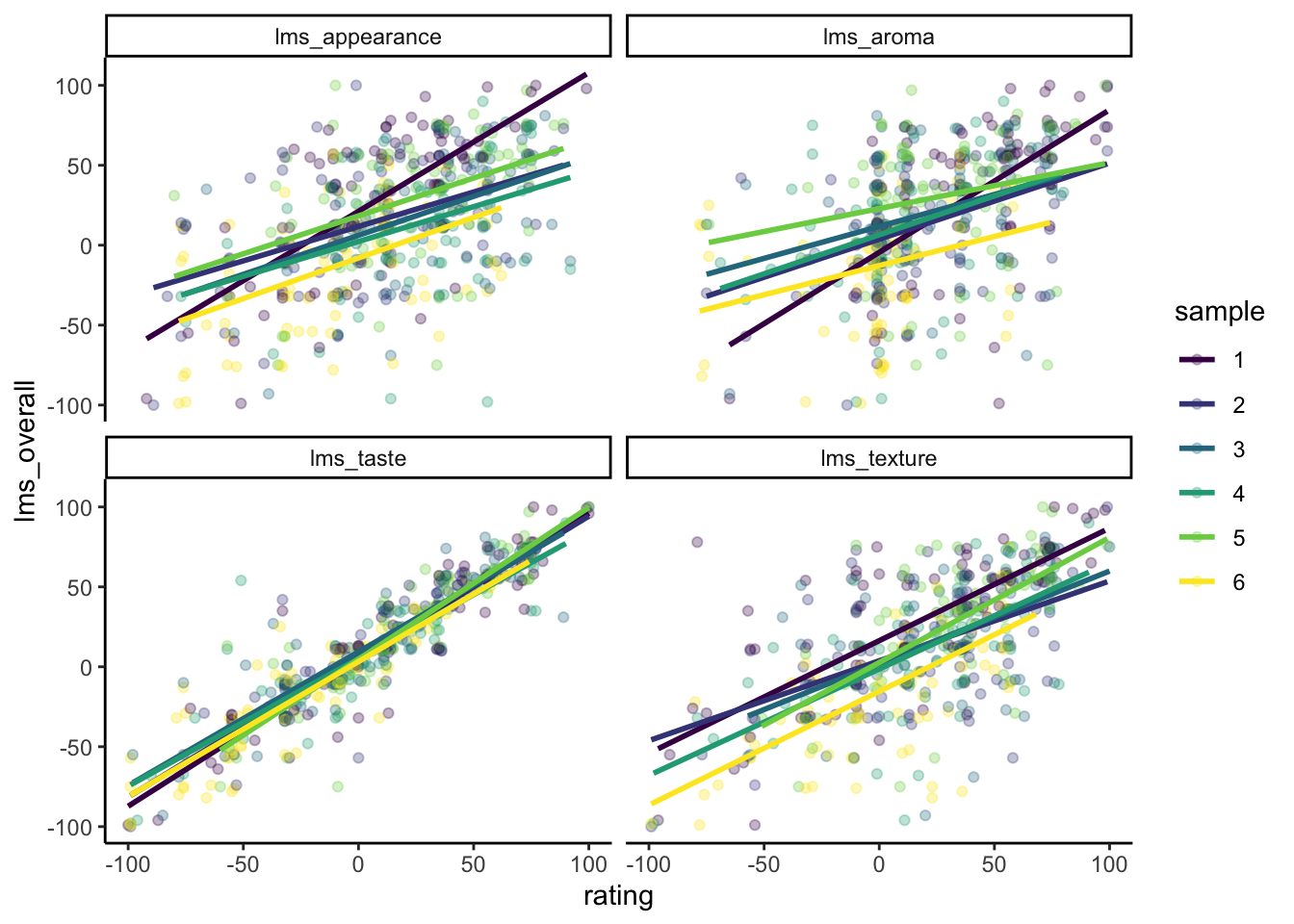

We can see that the response of sample 1 is quite different than the others for lms_appearance and lms_aroma. It seems like being rated higher on those attributes has a larger effect on lms_overall for sample 1 than for the other 5 samples.

ggplotly(p)

We can use this widget to explore these data for further hypotheses. Specifically, when we split up the data at the levels of different categorical variables and investigate other variables, we are exploring simple effects. These are the subject of the last topic we will explore–a simple machine-learning approach called Categorization, Partition, or Regression Trees.

But, before we move there, let’s have…

10.4 Some notes of caution on model selection

We’ve been talking about terms like “model selection”, which are jargon-y, so let’s refocus on what we’re doing: we are answering the question of “what of our experimental variables actually matter in explaining or predicting an outcome we care about?” In our example, we are asking, “if we ask people a lot of questions about berries, which ones are most related to how much they say they like each berry?”

I’ve shown off some powerful, data-based approaches to letting an algorithm decide on which variables to include in the model. Why don’t we just use these and make the process “objective”? While we will be getting into this question in detail next week, here are several things to consider:

Just remember the following: we are making predictions from data, not explaining causality.
Without a theory that explains why any relationship is one we would expect to see, we run into the problem of just letting our coincidence-finding systems make up a story for us, which leads us to…
Without expertise, we are just exploting patterns in the data that are quite possibly either accidental or are caused by a third, underlying variable. Remember the shark-attack example?
The reason we cannot use “objective” processes is that, unfortunately, objectivity doesn’t exist! At least, not in the way we wish it did. For example, our step() function minimizes the AIC, which is the Akaike Information Criterion. This isn’t some universal constant that exists–it is a relationship derived from the Maximum Likelihood Estimate of a model with the number of parameters in the model. Essentially, this expresses a human hypothesis of what makes a model function well. But there are other criteria we could minimize that instantiate different arguments. Just because something is a number doesn’t mean it is objective.

10.5 Categorization and Regression Trees (CART): A data-based approach

We’re going to end today with a machine-learning technique that combines and generalizes the tools of multi-way ANOVA, multiple regression, and stepwise model fitting we’ve been exploring today. We’re just going to dip our toes into so-called Categorization and Regression Trees (CART from now on) today, but I hope this will motivate you to examine them as a tool to use yourself.

Practical Statistics for Data Scientists (Bruce and Bruce 2017, 220–30) gives an excellent introduction to this topic, and it will be part of the reading this week. Very briefly, CART is appealing because:

It generates a simple, explanatory set of explanatory rules for explaining an outcome variable in a dataset that are easily communicated to a broad audience.
The outcome variable being explained can be either continuous (a regression tree) or categorical (a categorization tree) without loss of generality in the model.
Trees form the basis for more advanced, powerful machine-learning models such as Random Forest or Boosted Tree models which are among some of the most powerful and accessible models for machine learning.
In general, CART models can be made to fit any kind of data without relying on the (generally wrong) assumptions of traditional linear models.

So how does a tree work? Let’s take a look at two examples.

10.5.1 Regression trees

First, we’ll begin by applying a tree approach to the same task we’ve been exploring in berry_data–predicting lms_overall from the best set of predictor variables. We will use some new packages for this: rpart, rpart.plot, and partykit.

We will take a very similar approach to our stepwise model fitting, in that we will give the CART model a large set of variables to predict lms_overall from. We are going to use just our CATA and categorical data because it will make a more interesting tree, but in reality we’d want to include all variables we think might reasonably matter.

tree_data <- berry_data %>%
  select(-subject, -lms_appearance, -lms_aroma, -lms_taste, -lms_texture)

reg_cart <- rpart(formula = lms_overall ~ ., data = tree_data)
reg_cart

## n= 510 
## 
## node), split, n, deviance, yval
##       * denotes terminal node
## 
##  1) root 510 897147.10  15.290200  
##    2) cata_taste_berry< 0.5 275 383234.50  -7.072727  
##      4) cata_taste_fermented>=0.5 54  85208.00 -31.000000 *
##      5) cata_taste_fermented< 0.5 221 259556.70  -1.226244  
##       10) cata_taste_fruity< 0.5 165 182430.80  -5.969697 *
##       11) cata_taste_fruity>=0.5 56  62474.50  12.750000 *
##    3) cata_taste_berry>=0.5 235 215448.40  41.459570  
##      6) cata_taste_fruity< 0.5 83  92591.23  28.903610 *
##      7) cata_taste_fruity>=0.5 152 102626.80  48.315790  
##       14) sample=2,4,6 59  44403.80  38.372880 *
##       15) sample=1,3,5 93  48689.83  54.623660 *

What this “stem and leaf” output tells us is how the data is split. In a CART, each possible predictor is examined for the largest effect size (mean difference) in the outcome variable (lms_overall). Then, the data are split according to that predictor, and the process is carried out again on each new dataset (this is called a “recursive” process). This continues until a stopping criterion is met. Usually stopping is either number of observations (rows) in the final “leaves” of the tree, but there are a number of possibilities.

When we are predicting a continuous outcome like lms_overall, the test at each step is a simple ANOVA.

This is probably easier envisioned as a diagram:

reg_cart %>%
  rpart.plot(type = 5, extra = 101)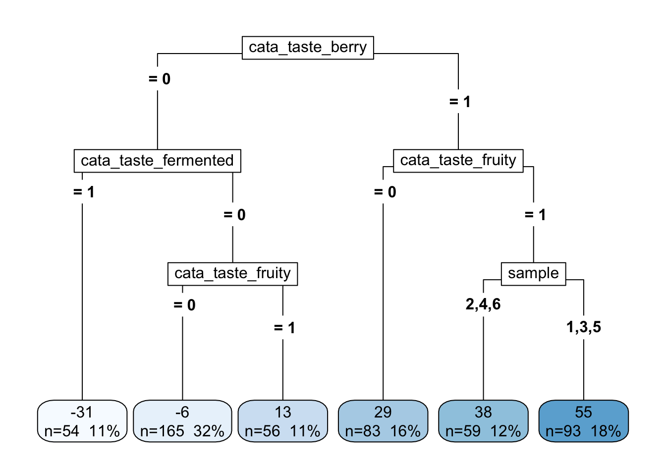

The “decision tree” output of this kind of model is a big part of it’s appeal. We can see that the most important predictor here is whether a subject has checked the CATA “berry” attribute. But after that, the next most important attribute is different. If there’s no “berry” flavor, it matters whether the sample is “fermented”, but if there is a berry flavor, then it matters whether it is “fruity”. And so on. In the terminal “leaves” we see the average rating for that combination of attributes as well as the number of samples that falls into that leaf.

We can also use the partykit plotting functions to get some different output:

reg_cart %>%
  as.party %>%
  plot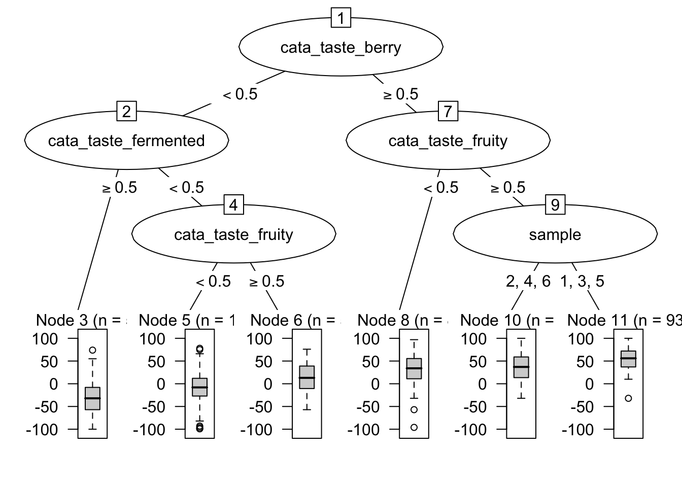

I present this largely because it is possible (but somewhat complicated) to use partykit with the package ggparty to construct these plots within ggplot2, but I won’t be getting into it (because it is still very laborious for me).

10.5.2 Categorization trees

In general, we cannot use a regression model to fit categorical outcomes (this is where we would get into logistic regression or other methods that use a transformation, which fall into the general linear model). However, CART models happily will predict a categorical outcome based on concepts of “homogeneity” and “impurity”–essentially, the model will try to find the splitting variables that end up with leaves having the most of one category of outcomes.

Here, we are going to do something conceptually odd: we’re going to predict sample from all of our other variables. We’re going to do this for two reasons:

This is actually an interesting question: we are asking what measured variables best separate our samples.
This emphasizes the fact that our data is almost entirely observational: in general we should be careful about forming conclusions (as opposed to further hypotheses) from these kinds of data, because our variables do not have one-way causal relationships.

catt_data <- berry_data %>%
  select(-subject)

cat_tree <- rpart(sample ~ ., data = catt_data)
cat_tree

## n= 510 
## 
## node), split, n, loss, yval, (yprob)
##       * denotes terminal node
## 
##  1) root 510 425 1 (0.17 0.17 0.17 0.17 0.17 0.17)  
##    2) lms_aroma>=12.5 237 178 1 (0.25 0.17 0.18 0.12 0.21 0.072)  
##      4) lms_appearance< 47.5 170 119 1 (0.3 0.2 0.12 0.11 0.19 0.082)  
##        8) lms_overall>=50.5 60  30 1 (0.5 0.15 0.13 0.067 0.12 0.033) *
##        9) lms_overall< 50.5 110  84 5 (0.19 0.23 0.11 0.13 0.24 0.11)  
##         18) lms_appearance< -55 10   4 2 (0.1 0.6 0.1 0.2 0 0) *
##         19) lms_appearance>=-55 100  74 5 (0.2 0.19 0.11 0.12 0.26 0.12)  
##           38) cata_taste_grassy>=0.5 35  25 2 (0.11 0.29 0.11 0.23 0.17 0.086) *
##           39) cata_taste_grassy< 0.5 65  45 5 (0.25 0.14 0.11 0.062 0.31 0.14)  
##             78) lms_aroma>=56.5 18  12 1 (0.33 0.22 0.22 0.056 0.056 0.11) *
##             79) lms_aroma< 56.5 47  28 5 (0.21 0.11 0.064 0.064 0.4 0.15) *
##      5) lms_appearance>=47.5 67  44 3 (0.12 0.09 0.34 0.15 0.25 0.045)  
##       10) lms_overall>=53.5 37  25 5 (0.19 0.081 0.16 0.24 0.32 0)  
##         20) lms_taste>=75.5 9   4 1 (0.56 0 0.11 0.33 0 0) *
##         21) lms_taste< 75.5 28  16 5 (0.071 0.11 0.18 0.21 0.43 0) *
##       11) lms_overall< 53.5 30  13 3 (0.033 0.1 0.57 0.033 0.17 0.1) *
##    3) lms_aroma< 12.5 273 205 6 (0.095 0.16 0.15 0.21 0.13 0.25)  
##      6) lms_appearance>=-9.5 180 130 4 (0.067 0.13 0.2 0.28 0.16 0.17)  
##       12) cata_taste_berry>=0.5 66  49 5 (0.14 0.11 0.23 0.17 0.26 0.11) *
##       13) cata_taste_berry< 0.5 114  75 4 (0.026 0.15 0.18 0.34 0.096 0.2) *
##      7) lms_appearance< -9.5 93  55 6 (0.15 0.23 0.065 0.075 0.075 0.41) *

Again, this will be easier to see if we plot it:

cat_tree %>%
  rpart.plot(type = 5, extra = 101)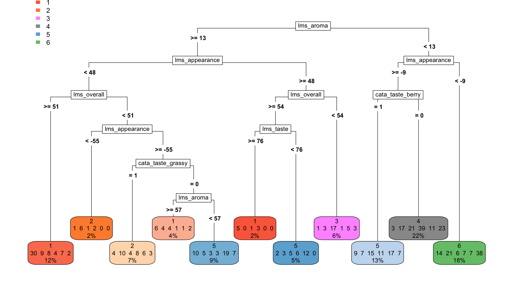

Figuring out how to plot this requires a fair amount of fiddling, but ultimately we are able to speak to how differences in many, interacting variables lead us to groups that are majority one type of sample.

10.6 Wrap-up

Today, we’ve spent our time on methods for understanding how multiple factors (variables) can be related to an outcome variable. We’ve moved from familiar models like ANOVA and regression to a more complex, machine-learning based approach (CART). What these models all have in common is that they attempt to explain a single outcome variable based on many possible predictors. We’ve just scratched the surface of this topic, and for your own work you’ll want to learn about both discipline-specific expectations for methods and what kind of approaches make sense for your own data. Also, this list will be important:

Are you trying to predict:

A single outcome from multiple categorical or continuous variables? Great! We did this!
Multiple outcomes from multiple continuous or categorical variables? You’re going to need multivariate stats (MANOVA, PCA, etc).
No outcomes, just trying to find patterns in your variables? You’re going to need machine learning (cluster analysis, PCA, etc).

As should be clear from this little list, we’ve only just, just, just started to scratch the surface. But I hope this will make you feel confident that you can learn these tools and apply them as needed. No one, including me, is an expert in all of these approaches. The key is to learn the basic rules and learn as much as you need to accomplish whatever your current goals are!

References

Bruce, Peter, and Andrew Bruce. 2017. Practical Statistics for Data Scientists. Sebastopol: O’Reilly.

Howell, David C. 2010. Statistical Methods for Psychology. 7th ed. Australia : Belmont, CA: Thomson Wadsworth.