5 Text Analysis

At this point we’ve gone over the fundamentals of data wrangling and analysis in R. We really haven’t touched on statistics and modeling, as that is outside the scope of this workshop, but I will be glad to chat about those with anyone outside of the main workshop if you have questions.

Now we’re going to turn to our key focus: text analysis in R. We are going to focus on 3 broad areas:

Importing, cleaning, and wrangling text data and dealing with character type data.
Basic text modeling using the TF-IDF framework
Application: Sentiment Analysis

It’s not a bad idea to restart your R session here. Make sure to save your work, but a clean Environment is great when we’re shifting topics.

You can accomplish this by going to Session > Restart R in the menu.

Then, we want to make sure to re-load our packages and import our data.

# The packages we're using
library(tidyverse)
library(tidytext)

# The dataset
beer_data <- read_csv("data/ba_2002.csv")

## Rows: 20359 Columns: 14
## ── Column specification ────────────────────────────────────────────────────────
## Delimiter: ","
## chr (5): reviews, beer_name, brewery_name, style, user_id
## dbl (9): beer_id, brewery_id, abv, appearance, aroma, palate, taste, overall...
## 
## ℹ Use `spec()` to retrieve the full column specification for this data.
## ℹ Specify the column types or set `show_col_types = FALSE` to quiet this message.

5.1 Text Analysis Pt. I: Getting your text data

There are many sources of text data, which is one of the strengths of this approach. Some quick and obvious examples include:

Open-comment responses on a survey (sensory study in lab, remote survey, etc)
Comment cards or customer responses
Qualitative data (transcripts from interviews and focus groups)
Compiled/database from previous studies
Scraped data from websites and/or social media

The last (#5) is often the most interesting data source, and there are a number of papers in recent years that have discussed the use of this sort of data. I am not going to discuss how to obtain text data in this presentation, because it is its own, rich topic. However, you can review my presentation and tutorial from Eurosense 2020 if you want a quick crash course on web scraping for sensory evaluation.

5.1.1 Basic import and cleaning with text data

So far we’ve focused our attention on the beer_data data set on the various (numeric) rating variables. But the data in the reviews column is clearly more rich.

set.seed(2)

reviews_example <- 
  beer_data %>%
  slice_sample(n = 5)

reviews_example %>%
  select(beer_name, reviews) %>%
  gt::gt()

beer_name	reviews
Stoudt's Weizen	Medium straw and cloudy with thick head and lace. Fresh smelling with slight lemon zest aroma. Taste is rich and fulfilling with strong lemon flavor. Also notable is the strong, almost overwhealming clove flavor. Fresh and thirst quenching. Goes great with brats at a German festival.
Black Bear Ale	(3-31-03): Got a new bottle thanks to johnrobe, and unfortunately it was just as bad. This brewery either has ongoing issues or the beer is really supposed to taste this way. I am guessing it is the former. (12-09-02): Acquired via trade. This may be a good beer and I may have gotten a bad bottle but the vinegar aroma ruined this beer. I was given pause before I even had a chance to take a sip because the vinegar aroma is so potent. Plugging my nose and drinking did not help much as the vinegar was prevalent in the flavor as well. I will give this one another shot down the road but I had to pour this one out.
Kozel	A truly good, authentic Pilsner, bordering on great. This is the type of Pilsner Beck's or Labatts (and most North American brewers) wished they could produce. They can't, this brew took time. Brew time and cellar time. The quality of ingredients and process are there for the palate to enjoy on this Pilsner. Soft barley and malt tastes balanced with those heavenly saaz bitters. A great example of Czech pilsen style lagers. This one has a distinguishing quality though. It has everything required of a good Pilsner, flowery hopping evident to the nose and palate, sharp crisp start, tart/malty/grassy in the mouth dry finish except, this one has no lingering "tinny" taste to the tongue from the saaz hops....probably not pasteurized. I liked this Pilsner very much and that takes something for this fanatical "Pils head". The only draw back is the price. $2.85 per 500mil bottle. I was surprised this beer was so fresh tasting, date code was near expired and it sat unrefrigerated on the LCBO (our state liquor monopoly) shelf. A must try if you like Pilsners.
Odell Cutthroat Pale Ale	This beer pours with a deep thick copper color and a thick foamy white head. The huge spicy aroma has just a hint of malt. The smooth medium body initiates an up-front caramel malt sweetness followed by a sharp spicy bitter bite. Very tasty.
Pike XXXXX Stout	Nice pour, deep opaque black with an easy, thick creamy head that clings to the sides of the glass. It's not exactly long-lasting, but it never fully fades (ends up thin cream layer that's too thick for a film, but kind of like a like coat of moss or lichens). The aroma is a little weak, but roasty. The flavor is as strong as it should be but it dominated and unbalanced by too much burned bitterness. A bit of smokiness lingers underneath. The lack of balance makes this less than a joy to drink, but intriguing at the same time.

However, this has some classic features of scraped text data–notice the “&quot”, for example–this is HTML placeholder for a quotation mark. Other common problems that you will see with text data include “parsing errors” between different forms of character data–the most common is between ASCII and UTF-8 standards. You will of course also encounter errors with typos, and perhaps idiosyncratic formatting characteristic of different text sources: for example, the use of @usernames and #hashtags in Twitter data.

We will use the textclean package to do some basic clean up, but this kind of deep data cleaning may take more steps and will change from project to project.

library(textclean)

cleaned_reviews_example <- 
  reviews_example %>%
  mutate(cleaned_review = reviews %>%
           # Fix some of the HTML placeholders
           replace_html(symbol = FALSE) %>%
           # Replace sequences of "..." 
           replace_incomplete(replacement = " ") %>%
           # Replace less-common or misformatted HTML
           str_replace_all("#.{1,4};", " ") %>%
           # Replace some common non-A-Z, 1-9 symbols
           replace_symbol() %>% 
           # Remove non-word text like ":)"
           replace_emoticon() %>%
           # Remove numbers from the reviews, as they are not useful
           str_remove_all("[0-9]"))

cleaned_reviews_example %>%
  select(beer_name, cleaned_review) %>%
  gt::gt()

beer_name	cleaned_review
Stoudt's Weizen	Medium straw and cloudy with thick head and lace. Fresh smelling with slight lemon zest aroma. Taste is rich and fulfilling with strong lemon flavor. Also notable is the strong, almost overwhealming clove flavor. Fresh and thirst quenching. Goes great with brats at a German festival.
Black Bear Ale	(--): Got a new bottle thanks to johnrobe, and unfortunately it was just as bad. This brewery either has ongoing issues or the beer is really supposed to taste this way. I am guessing it is the former. (--): Acquired via trade. This may be a good beer and I may have gotten a bad bottle but the vinegar aroma ruined this beer. I was given pause before I even had a chance to take a sip because the vinegar aroma is so potent. Plugging my nose and drinking did not help much as the vinegar was prevalent in the flavor as well. I will give this one another shot down the road but I had to pour this one out.
Kozel	A truly good, authentic Pilsner, bordering on great. This is the type of Pilsner Beck's or Labatts (and most North American brewers) wished they could produce. They can't, this brew took time. Brew time and cellar time. The quality of ingredients and process are there for the palate to enjoy on this Pilsner. Soft barley and malt tastes balanced with those heavenly saaz bitters. A great example of Czech pilsen style lagers. This one has a distinguishing quality though. It has everything required of a good Pilsner, flowery hopping evident to the nose and palate, sharp crisp start, tart/malty/grassy in the mouth dry finish except, this one has no lingering tinny taste to the tongue from the saaz hops probably not pasteurized. I liked this Pilsner very much and that takes something for this fanatical Pils head . The only draw back is the price. dollar . per mil bottle. I was surprised this beer was so fresh tasting, date code was near e tongue sticking out ired and it sat unrefrigerated on the LCBO (our state liquor monopoly) shelf. A must try if you like Pilsners.
Odell Cutthroat Pale Ale	This beer pours with a deep thick copper color and a thick foamy white head. The huge spicy aroma has just a hint of malt. The smooth medium body initiates an up-front caramel malt sweetness followed by a sharp spicy bitter bite. Very tasty.
Pike XXXXX Stout	Nice pour, deep opaque black with an easy, thick creamy head that clings to the sides of the glass. It's not exactly long-lasting, but it never fully fades (ends up thin cream layer that's too thick for a film, but kind of like a like coat of moss or lichens). The aroma is a little weak, but roasty. The flavor is as strong as it should be but it dominated and unbalanced by too much burned bitterness. A bit of smokiness lingers underneath. The lack of balance makes this less than a joy to drink, but intriguing at the same time.

This will take slightly longer to run on the full data set, but should improve our overall data quality.

beer_data <- 
  beer_data %>%
  mutate(cleaned_review = reviews %>%
           replace_html(symbol = FALSE) %>%
           replace_incomplete(replacement = " ") %>%
           str_replace_all("#.{1,4};", " ") %>%
           replace_symbol() %>%
           replace_emoticon() %>%
           str_remove_all("[0-9]"))

Again, this is not an exhaustive cleaning step–rather, these are some basic steps that I took based on common parsing errors I observed. Each particular text dataset will come with its own challenges and require a bit of time to develop the cleaning step.

5.1.2 Where is the data in `character`? A tidy approach.

As humans who understand English, we can see that meaning is easily found from these reviews. For example, we can guess that the rating of Black Bear Ale will be a low number (negative), while the rating of Kozel will be much more positive. And, indeed, this is the case:

cleaned_reviews_example %>% 
  select(beer_name, appearance:rating)

## # A tibble: 5 × 7
##   beer_name                appearance aroma palate taste overall rating
##   <chr>                         <dbl> <dbl>  <dbl> <dbl>   <dbl>  <dbl>
## 1 Stoudt's Weizen                 4     3.5    4     4       4     3.88
## 2 Black Bear Ale                  3     1      1     1.5     1.5   1.42
## 3 Kozel                           4     4      4.5   4.5     4     4.25
## 4 Odell Cutthroat Pale Ale        4     4      4     4       4     4   
## 5 Pike XXXXX Stout                4.5   3      4     3.5     2.5   3.29

But what part of the structure of the reviews text actually tells us this? This is a complicated topic that is well beyond the scope of this workshop–we are going to propose a single approach based on tokenization that is effective, but is certainly not exhaustive.

If you are interested in a broader view of approaches to text analysis, I recommend the seminal textbook from Jurafsky and Martin, Speech and Language Processing, especially chapters 2-6. The draft version is freely available on the web as of the date of this workshop.

In the first half of this workshop we reviewed the tidyverse approach to data, in which we emphasized an approach to data in which:

Each variable is a column

Each observation is a row

Each type of observational unit is a table

This type of approach can be applied to text data if we can specify a way to standardize the “observations” within the text. We will be applying and demonstrating the approach defined and promoted by Silge and Robinson in Text Mining with R, in which we will focus on the following syllogism to create tidy text data:

observation == token

A token is a meaningful unit of text, usually but not always a single word, which will be the observation for us. In our example data, let’s identify some possible tokens:

cleaned_reviews_example$cleaned_review[1]

## [1] "Medium straw and cloudy with thick head and lace. Fresh smelling with slight lemon zest aroma. Taste is rich and fulfilling with strong lemon flavor. Also notable is the strong, almost overwhealming clove flavor. Fresh and thirst quenching. Goes great with brats at a German festival."

We will start with only examining single words, also called “unigrams” in the linguistics jargon. Thus, Medium, straw, and cloudy are the first tokens in this dataset. We will mostly ignore punctuation and spacing, which means we are giving up some meaning for convenience.

We could figure out how to manually break this up into tokens with enough work, using functions like str_separate(), but happily there are a large set of competing R tools for tokenization, for example:

cleaned_reviews_example$cleaned_review[1] %>%
  tokenizers::tokenize_words(simplify = TRUE)

##  [1] "medium"        "straw"         "and"           "cloudy"       
##  [5] "with"          "thick"         "head"          "and"          
##  [9] "lace"          "fresh"         "smelling"      "with"         
## [13] "slight"        "lemon"         "zest"          "aroma"        
## [17] "taste"         "is"            "rich"          "and"          
## [21] "fulfilling"    "with"          "strong"        "lemon"        
## [25] "flavor"        "also"          "notable"       "is"           
## [29] "the"           "strong"        "almost"        "overwhealming"
## [33] "clove"         "flavor"        "fresh"         "and"          
## [37] "thirst"        "quenching"     "goes"          "great"        
## [41] "with"          "brats"         "at"            "a"            
## [45] "german"        "festival"

Note that this function also (by default) turns every word into its lowercase version (e.g., Medium becomes medium) and strips out punctuation. This is because, to a program like R, upper- and lowercase versions of the same string are not equivalent. If we have reason to believe preserving this difference is important, we might want to rethink allowing this behavior.

Now, we have 46 observed tokens for our first review in our example dataset. But of course this is not super interesting–we need to apply this kind of transformation to every single one of our ~20,000 reviews. With some fiddling around with mutate() we might be able to come up with a solution, but happily this is where we start using the tidytext package. The unnest_tokens() function built into that package will allow us to transform our text directly into the format we want, with very little effort.

beer_data_tokenized <-
  beer_data %>%
  # We may want to keep track of a unique ID for each review
  mutate(review_id = row_number()) %>%
  unnest_tokens(output = token,
                input = cleaned_review,
                token = "words") %>%
  # Here we do a bit of extra cleaning
  mutate(token = str_remove_all(token, "\\.|_"))

beer_data_tokenized %>%
  # We show just a few of the columns for printing's sake
  select(beer_name, rating, token)

## # A tibble: 1,770,136 × 3
##    beer_name           rating token
##    <chr>                <dbl> <chr>
##  1 Caffrey's Irish Ale   4.46 this 
##  2 Caffrey's Irish Ale   4.46 is   
##  3 Caffrey's Irish Ale   4.46 a    
##  4 Caffrey's Irish Ale   4.46 very 
##  5 Caffrey's Irish Ale   4.46 good 
##  6 Caffrey's Irish Ale   4.46 irish
##  7 Caffrey's Irish Ale   4.46 ale  
##  8 Caffrey's Irish Ale   4.46 i'm  
##  9 Caffrey's Irish Ale   4.46 not  
## 10 Caffrey's Irish Ale   4.46 sure 
## # … with 1,770,126 more rows
## # ℹ Use `print(n = ...)` to see more rows

The unnest_tokens() function actually applies the tokenizers::tokenize_words() function in an efficient, easy way: it takes a column of raw character data and then tokenizes it as specified, outputting a tidy format of 1-token-per-row. Now we have our observations (tokens) each on its own line, ready for further analysis.

In order to make what we’re doing easier to follow, let’s also take a look at our example data.

cleaned_reviews_tokenized <- 
  cleaned_reviews_example %>%
  unnest_tokens(input = cleaned_review, output = token) %>%
  # Here we do a bit of extra cleaning
  mutate(token = str_remove_all(token, "\\.|_"))

cleaned_reviews_tokenized %>%
  filter(beer_name == "Kozel") %>%
  # Let's select a few variables for printing
  select(beer_name, rating, token)

## # A tibble: 187 × 3
##    beer_name rating token    
##    <chr>      <dbl> <chr>    
##  1 Kozel       4.25 a        
##  2 Kozel       4.25 truly    
##  3 Kozel       4.25 good     
##  4 Kozel       4.25 authentic
##  5 Kozel       4.25 pilsner  
##  6 Kozel       4.25 bordering
##  7 Kozel       4.25 on       
##  8 Kozel       4.25 great    
##  9 Kozel       4.25 this     
## 10 Kozel       4.25 is       
## # … with 177 more rows
## # ℹ Use `print(n = ...)` to see more rows

When we use unnest_tokens(), all of the non-text data gets treated as information about each token–so beer_name, rating, etc are duplicated for each token that now has its own row. This will allow us to perform a number of types of text analysis.

5.1.3 A quick note: saving data

We’ve talked about wanting to clear our workspace from R in between sessions to make sure our work and code are reproducible. But at this point we’ve done a lot of work, and we might want to save this work for later. Or, we might want to share our work with others. The tidyverse has a good utility for this when we’re working with data frames and tibbles: the write_csv() function is the opposite of the read_csv() function we’ve gotten comfortable with: it takes a data frame and writes it into a .csv file that is easily shared with others or reloaded in a later session.

# Let's store our cleaned and tokenized reviews
write_csv(x = beer_data_tokenized, file = "data/tokenized_beer_reviews.csv")

5.2 Text Analysis Pt. II: Basic text analysis approaches using tokens

We’ve now seen how to import and clean text, and to transform text data into one useful format for analysis: a tidy table of tokens. (There are certainly other useful formats, but we will not be covering them here.)

Now we get to the actually interesting part. We’re going to tackle some basic but powerful approaches for parsing the meaning of large volumes of text.

5.2.1 Word counts

A common approach for getting a quick, analytic summary of the nature of the tokens (observations) in our reviews might be to look at the frequency of word use across reviews: this is pretty closely equivalent to a Check-All-That-Apply (CATA) framework: we will look how often each term is used, and will then extend this to categories of interest to our analysis. So, for example, we might have hypotheses like the following that we could hope to investigate using word frequencies:

Overall, flavor words are the most frequently used words in reviews of beer online.
The frequency of flavor-related words will be different for major categories of beer, like “hop”-related words for IPAs and “chocolate”/“coffee” terms for stouts.
The top flavor words will be qualitatively more positive for reviews associated with the top 10% of ratings, and negative for reviews associated with the bottom 10%.

I will not be exploring each of these in this section of the workshop because of time constraints, but hopefully you’ll be able to use the tools I will demonstrate to solve these problems on your own.

Let’s start by combining our tidy data wrangling skills from tidyverse with our newly tidied text data from unnest_tokens() to try to test the first answer.

beer_data_tokenized %>%
  # The count() function gives the number of rows that contain unique values
  count(token) %>%
  # get the 20 most frequently occurring words
  slice_max(order_by = n, n = 20) %>%
  # Here we do some wrangling for visualization
  mutate(token = as.factor(token) %>% fct_reorder(n)) %>%
  # let's visualize this just for fun
  ggplot(aes(x = token, y = n)) + 
  geom_col() + 
  coord_flip() + 
  theme_bw() +
  labs(x = NULL, y = NULL, title = "The 20 most frequent words are not that useful.")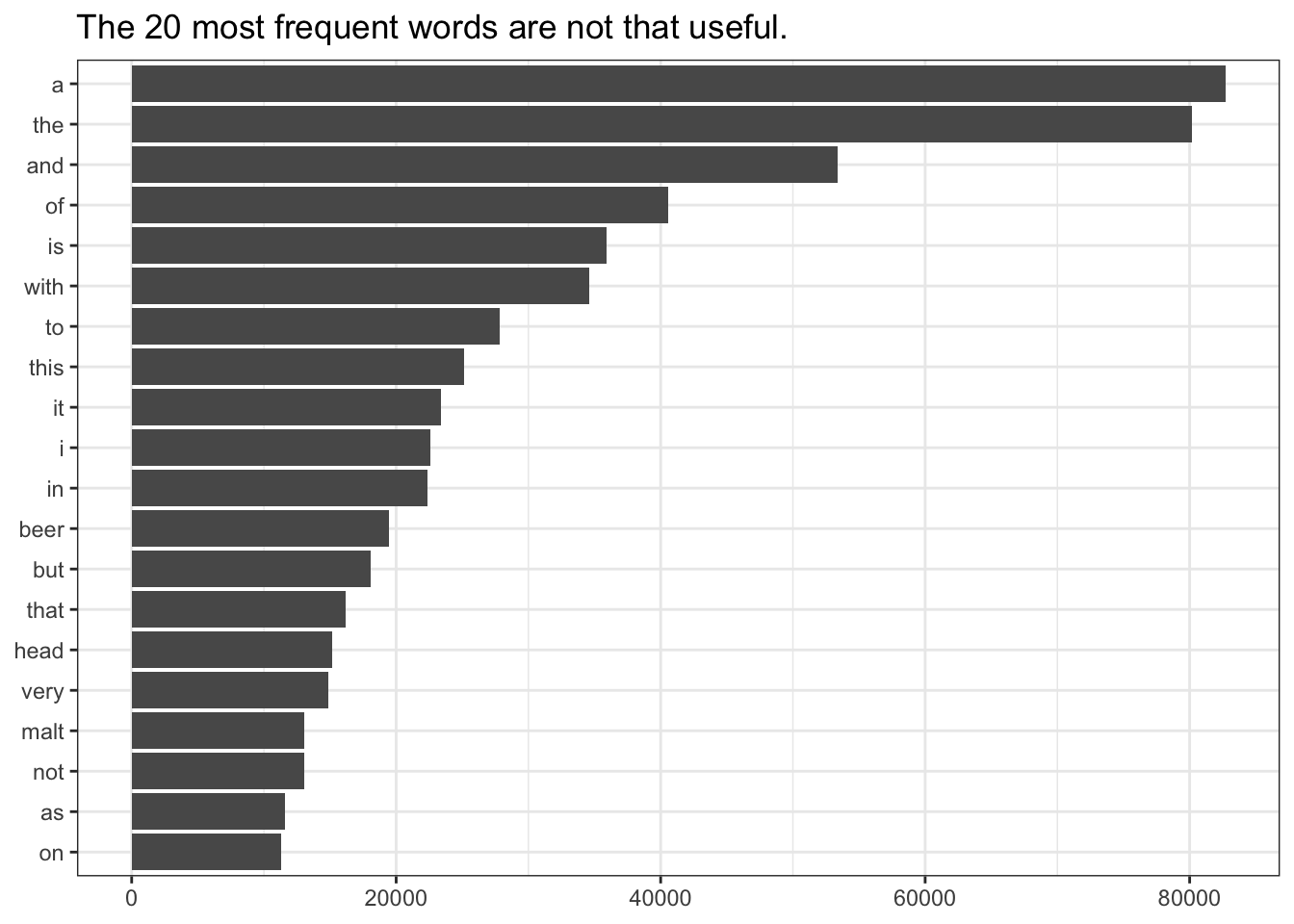

Unfortunately for our first hypothesis, we have quickly encountered a common problem in token-based text analysis. The most frequent words in most languages are “helper” words that are necessary for linguistic structure and communication, but are not unique to a particular topic or context. For example, in English the articles a, and the tend to be the most frequent tokens in any text because they are so ubiquitous.

It takes us until the 15th most frequent word, head, to find a word that might have sensory or product implications.

So, in order to find meaning in our text, we need to find some way to look past these terms, whose frequency vastly outnumbers words we are actually interested in.

5.2.1.1 “stop words”

In computational linguistics, this kind of word is often called a stop word: a word that is functionally important but does not tell us much about the meaning of the text. There are many common lists of such stop words, and in fact the tidytext package provides one such list in the stop_words tibble:

stop_words

## # A tibble: 1,149 × 2
##    word        lexicon
##    <chr>       <chr>  
##  1 a           SMART  
##  2 a's         SMART  
##  3 able        SMART  
##  4 about       SMART  
##  5 above       SMART  
##  6 according   SMART  
##  7 accordingly SMART  
##  8 across      SMART  
##  9 actually    SMART  
## 10 after       SMART  
## # … with 1,139 more rows
## # ℹ Use `print(n = ...)` to see more rows

The most basic approach to dealing with stop words is just to outright remove them from our data. This is easy when we’ve got a tidy, one-token-per-row structure.

We could use some version of filter() to remove stop words from our beer_data_tokenized tibble, but this is exactly what the anti_join() function (familiar to those of you who have used SQL) will do: with two tibbles, X and Y, anti_join(X, Y) will remove all rows in X that match rows in Y.

beer_data_tokenized %>%
  # "by = " tells what column to look for in X and Y
  anti_join(y = stop_words, by = c("token" = "word")) %>%
  count(token) %>%
  # get the 20 most frequently occurring words
  slice_max(order_by = n, n = 20) %>%
  # Here we do some wrangling for visualization
  mutate(token = as.factor(token) %>% fct_reorder(n)) %>%
  # let's visualize this just for fun
  ggplot(aes(x = token, y = n)) + 
  geom_col() + 
  coord_flip() + 
  theme_bw() +
  labs(x = NULL, y = NULL, title = "These tokens are much more relevant.", subtitle = "We removed ~1200 stop words.")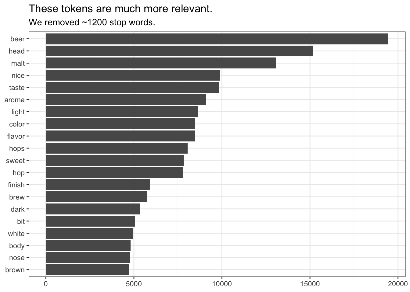

Now we are able to address our very first hypothesis: while the most common term (beer) might be in fact a stop word for this data set, the next 11 top terms all seem to have quite a lot to do with flavor.

We can extend this approach just a bit to provide the start of one answer to our second question: are there different most-used flavor terms for different beer styles? We can start to tackle this by first defining a couple of categories (since there are a lot of different styles in this dataset):

beer_data %>%
  count(style)

## # A tibble: 99 × 2
##    style                              n
##    <chr>                          <int>
##  1 Altbier                          186
##  2 American Adjunct Lager           961
##  3 American Amber / Red Ale         653
##  4 American Amber / Red Lager       235
##  5 American Barleywine              187
##  6 American Black Ale                10
##  7 American Blonde Ale              251
##  8 American Brown Ale               166
##  9 American Dark Wheat Ale           11
## 10 American Double / Imperial IPA   151
## # … with 89 more rows
## # ℹ Use `print(n = ...)` to see more rows

Let’s just look at the categories I suggested, plus “lager”. We will do this by using mutate to create a simple_style column:

# First, we'll make sure our approach works
beer_data %>%
  # First we will set our style to lower case to make matching easier
  mutate(style = tolower(style),
         # Then we will use a conditional match to create our new style
         simple_style = case_when(str_detect(style, "lager") ~ "lager",
                                  str_detect(style, "ipa") ~ "IPA",
                                  str_detect(style, "stout|porter") ~ "dark",
                                  TRUE ~ "other")) %>%
  count(simple_style)

## # A tibble: 4 × 2
##   simple_style     n
##   <chr>        <int>
## 1 dark          2562
## 2 IPA           1274
## 3 lager         3245
## 4 other        13278

# Then we'll implement the approach for our tokenized data
beer_data_tokenized <- 
  beer_data_tokenized %>%
  mutate(style = tolower(style),
         # Then we will use a conditional match to create our new style
         simple_style = case_when(str_detect(style, "lager") ~ "lager",
                                  str_detect(style, "ipa") ~ "IPA",
                                  str_detect(style, "stout|porter") ~ "dark",
                                  TRUE ~ "other")) 

# Finally, we'll plot the most frequent terms for each simple_style
beer_data_tokenized %>%
  # filter out stop words
  anti_join(stop_words, by = c("token" = "word")) %>%
  # This time we count tokens WITHIN simple_style
  count(simple_style, token) %>%
  # Then we will group_by the simple_style
  group_by(simple_style) %>%
  slice_max(order_by = n, n = 20) %>%
  # Removing the group_by is necessary for some steps
  ungroup() %>%
  # A bit of wrangling for plotting
  mutate(token = as.factor(token) %>% reorder_within(by = n, within = simple_style)) %>%
  ggplot(aes(x = token, y = n, fill = simple_style)) +
  geom_col(show.legend = FALSE) + 
  facet_wrap(~simple_style, scales = "free", ncol = 4) + 
  scale_x_reordered() + 
  theme_bw() + 
  coord_flip() +
  labs(x = NULL, y = NULL, title = "Different (sensory) words tend to be used with different styles.") +
  theme(axis.text.x = element_text(angle = 90))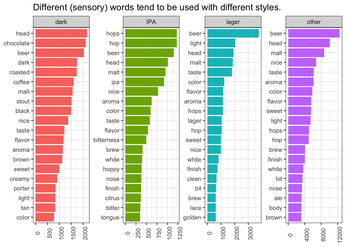

5.2.2 Term Frequency-Inverse Document Frequency (TF-IDF)

We have seen that removing stop words dramatically increases the quality of our analysis in regards to our specific answers. However, you may be asking yourself: “how do I know what counts as as a stop word?” For example, we see that “beer” is near the top of the list of most frequent tokens for all 4 categories we defined–it is not useful to us–but it is not part of the stop_words tibble. We could, of course, manually remove it (something like filter(token != "beer")). But removing each stop word manually requires us to make a priori judgments about our data, which is not ideal.

One approach that takes a statistical approach to identifying and filtering stop words without the need to define them a priori is the tf-idf statistic, which stands for Term Frequency-Inverse Document Frequency.

tf-idf requires not just defining tokens, as we have done already using the unnest_tokens() function, but defining “documents” for your specific dataset. The term “document” is somewhat misleading, as it is merely a categorical variable that tells us distinct units in which we want to compare the frequency of our tokens. So in our dataset, simple_style is one such document categorization (representing 4 distinct “documents”); we could also use style, representing 99 distinct categories (“documents”), or any other categorical variable.

The reason that we need to define a “document” variable for our dataset is that td-idf will answer, in general, the following question:

Given a set of “documents”, what tokens are most frequent within each unique document, but are not common between all documents?

Defined this way, it is clear that tf-idf has an empirical kinship with all kinds of within/between statistics that we use on a daily basis. In practice, tf-idf is a simple product of two empirical properties of each token in the dataset.

5.2.2.1 Term Frequency

The tf is defined simply for each combination of document and token as the raw count of that token in that document, divided by the sum of raw counts of all tokens in that document.

$\text{tf}(t, d) = \frac{count_{t}}{\sum_{t \in d}{count_{t}}}$

This quantity may be modified (for example, by using smoothing with $\log{(1 + count_{t})}$). Exact implementations can vary.

5.2.2.2 Inverse Document Frequency

The idf is an empirical estimate of how good a particular token is at distinguishing one “document” from another. It is defined as the logarithm of the total number of documents, divided by the the number of documents that contain the term in question.

$\text{idf}(t, D) = \log{\frac{N_D}{|\{{d \in D \ : \ t \in d\}|}}}$

Where $D$ is the set of documents in the dataset.

Remember that we obtain the tf-idf by multiplying the two terms, which explains the inverse fraction–if we imagined a “tf/df” with division, the definition of the document frequency might be more intuitive but less numerically tractable.

5.2.2.3 Applying tf-idf in `tidytext`

Overall, the tf part of tf-idf is just a scaled what we’ve been doing so far. But the idf part provides a measure of validation. For our very frequent terms, that we have been removing as stop words, the tf might be high (they occur a lot) but the idf will be extremely small–all documents use tokens like the and is, so they provide little discriminatory power between documents. Ideally, then, tf-idf will give us a way to drop out stop words without the need to specify them a priori.

Happily, we don’t have to figure out a function for calculating tf-idf ourselves; tidytext provides the bind_tf_idf() function. The only requirement is that we have a data frame that provides a per-“document” count for each token, which we have already done above:

# Let's first experiment with our "simple_styles"
beer_styles_tf_idf <-
  beer_data_tokenized %>%
  count(simple_style, token) %>%
  # And now we can directly add on tf-idf
  bind_tf_idf(term = token, document = simple_style, n = n)

beer_styles_tf_idf %>%
  # let's look at some stop words
  filter(token %in% c("is", "a", "the", "beer")) %>%
  gt::gt()

simple_style	token	n	tf
dark	a	10322	0.045447741
dark	beer	2041	0.008986518
dark	is	4682	0.020614835
dark	the	10610	0.046715804
IPA	a	5285	0.045000937
IPA	beer	1151	0.009800582
IPA	is	2364	0.020129085
IPA	the	5630	0.047938557
lager	a	11868	0.045791277
lager	beer	3773	0.014557675
lager	is	5628	0.021714974
lager	the	10734	0.041415872
other	a	55217	0.047339678
other	beer	12491	0.010709019
other	is	23222	0.019909122
other	the	53203	0.045612997

We can see that, despite very high raw counts for all of these terms, the tf-idf is 0! They do not discriminate across our document categories at all, and so if we start looking for terms with high tf-idf, these will drop out completely.

Let’s take a look at the same visualization we made before with raw counts, but now with tf-idf.

beer_styles_tf_idf %>%
  # We still group by simple_style
  group_by(simple_style) %>%
  # Now we want tf-idf, not raw count
  slice_max(order_by = tf_idf, n = 20) %>%
  ungroup() %>%
  # A bit of wrangling for plotting
  mutate(token = as.factor(token) %>% reorder_within(by = tf_idf, within = simple_style)) %>%
  ggplot(aes(x = token, y = tf_idf, fill = simple_style)) +
  geom_col(show.legend = FALSE) + 
  facet_wrap(~simple_style, scales = "free", ncol = 4) + 
  scale_x_reordered() + 
  theme_bw() + 
  coord_flip() +
  labs(x = NULL,
       y = NULL, 
       title = "With tf-idf we get much more specific terms.", 
       subtitle = "For example, 'oatmeal' for stouts, 'grapefruity' for IPAs, and so on.") +
  theme(axis.text.x = element_blank())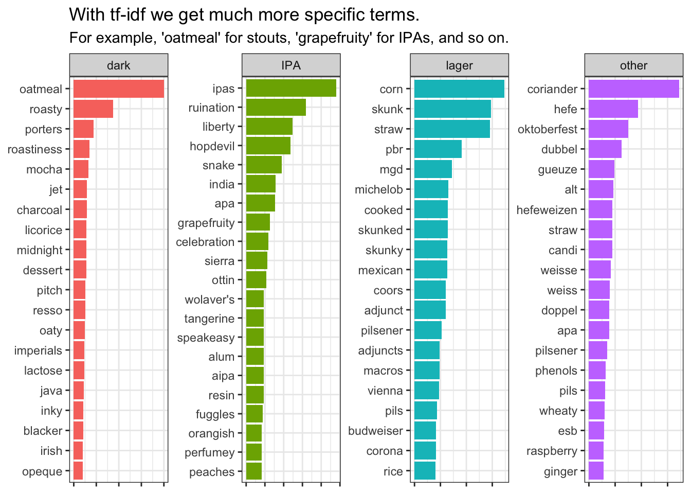

Thus, tf-idf gives us a flexible, empirical (data-based) model that will surface unique terms for us directly from the data. We can apply the same approach, for example, with a bit of extra wrangling, to see what terms are most associated with beers from the bottom and top deciles by rating (starting to address hypothesis #3):

beer_data_tokenized %>%
  # First we get deciles of rating
  mutate(rating_decile = ntile(rating, n = 10)) %>%
  # And we'll select just the top 2 and bottom 2 deciles %>%
  filter(rating_decile %in% c(1, 2, 9, 10)) %>%
  # Then we follow the exact same pipeline to get tf-idf
  count(rating_decile, token) %>%
  bind_tf_idf(term = token, document = rating_decile, n = n) %>%
  group_by(rating_decile) %>%
  # Since we have more groups, we'll just look at 10 tokens
  slice_max(order_by = tf_idf, n = 10) %>%
  ungroup() %>%
  # A bit of wrangling for plotting
  mutate(token = as.factor(token) %>% reorder_within(by = tf_idf, within = rating_decile)) %>%
  ggplot(aes(x = token, y = tf_idf, fill = rating_decile)) +
  geom_col(show.legend = FALSE) + 
  facet_wrap(~rating_decile, scales = "free", ncol = 4) + 
  scale_x_reordered() + 
  scale_fill_viridis_c() +
  theme_bw() + 
  coord_flip() +
  labs(x = NULL,
       y = NULL, 
       subtitle = "When we compare the top 2 and bottom 2 deciles, we see much more affective language.") +
  theme(axis.text.x = element_blank())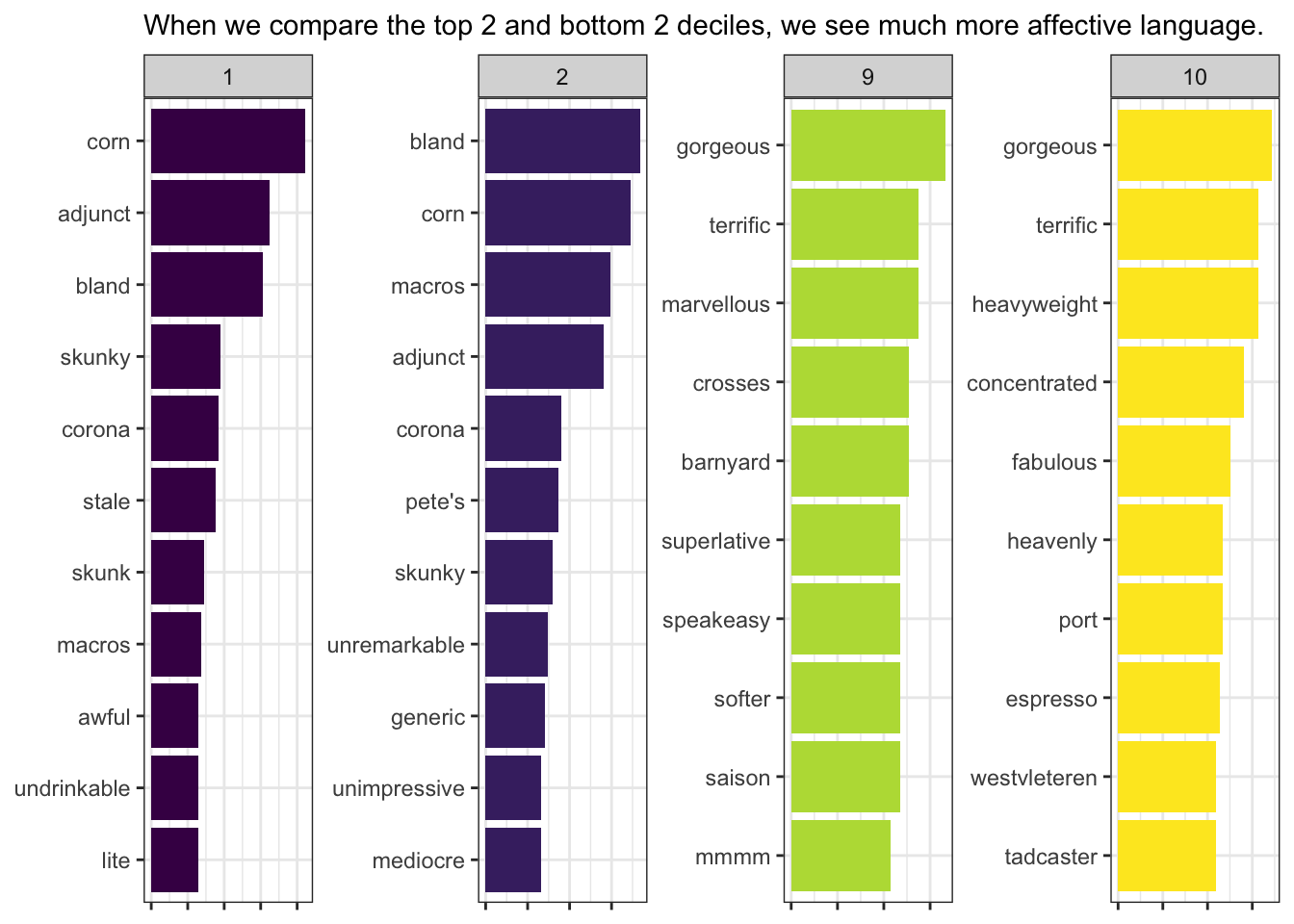

And important point to keep in mind about tf-idf is that it is data-based: the numbers are only meaningful within the specific set of tokens and documents. Thus, if I repeat the above pipeline but include all 10 deciles, we will not see the same words (and we will see that the model immediately struggles to find meaningful terms at all). This is because I am no longer calculating with 4 documents, but 10. These statistics are best thought of as descriptive, especially when we are repeatedly using them to explore a dataset.

We’ve now practiced some basic tools for first wrangling text data into a form with which we can work, and then applying some simple, empirical statistics to start to extract meaning. We’ll discuss sentiment analysis, a broad suite of tools that attempts to impute some sort of emotional or affective weight to words, and then produce scores for texts based on these weights.

5.3 Text Analysis Pt. III: Sentiment analysis

In recent years, sentiment analysis has gotten a lot of attention in consumer sciences, and it’s one of the topics that has penetrated the furthest into sensory science, because its goals are easily understood in terms of our typical goals: quantifying consumer affective responses to a set of products based on consumption experiences.

In sentiment analysis, we attempt to replicate the human inferential process, in which we, as readers, are able to infer–without necessarily being able to explicitly describe how we can tell–the emotional tone of a piece of writing. We understand implicitly whether the author is trying to convey various emotional states, like disgust, appreciation, joy, etc.

In recent years, there have been a number of approaches to sentiment analysis. The current state of the art is to use some kind of machine learning, such as random forests (“shallow learning”) or pre-trained neural networks (“deep learning”; usually convolutional, but sometimes recursive) to learn about a large batch of similar texts and then to process texts of interest. Not to plug myself too much, but we have a poster on such an approach at this conference, which may be of interest to some of you.

Machine learning: just throw algebra at the problem! (via XKCD)

While these state-of-the-art approaches are outside of the scope of this workshop, older techniques that use pre-defined dictionaries of sentiment words are easy to implement with a tidy text format, and can be very useful for the basic exploration of text data. These have been used in recent publications to great effect, such as in the recent paper from Luc et al. (2020).

The tidytext package includes the sentiments tibble by default, which is a version of that published by Hu & Liu (2004).

sentiments

## # A tibble: 6,786 × 2
##    word        sentiment
##    <chr>       <chr>    
##  1 2-faces     negative 
##  2 abnormal    negative 
##  3 abolish     negative 
##  4 abominable  negative 
##  5 abominably  negative 
##  6 abominate   negative 
##  7 abomination negative 
##  8 abort       negative 
##  9 aborted     negative 
## 10 aborts      negative 
## # … with 6,776 more rows
## # ℹ Use `print(n = ...)` to see more rows

count(sentiments, sentiment)

## # A tibble: 2 × 2
##   sentiment     n
##   <chr>     <int>
## 1 negative   4781
## 2 positive   2005

This is a very commonly used lexicon, which has shown to perform reasonably well on online-review based texts. The tidytext package also gives easy access to a few other lexicons through the get_sentiment() function, which may prompt for downloading some of the lexicons in order to avoid copyright issues. For the purpose of this workshop, we’ll just work with the sentiments tibble, which can also be accessed using get_sentiment("bing").

The structure of tidy data with tokens makes it very easy to use these dictionary-based sentiment analysis approaches. To do so, all we need to do is use a left_join() function, which is similar to the anti_join() function we used for stop words. In this case, for data tables X and Y, left_join(X, Y) finds rows in Y that match X, and imports all the columns from Y for those matches.

beer_sentiments <- 
  beer_data_tokenized %>%
  left_join(sentiments, by = c("token" = "word"))

beer_sentiments %>%
  select(review_id, beer_name, style, rating, token, sentiment)

## # A tibble: 1,770,138 × 6
##    review_id beer_name           style         rating token sentiment
##        <int> <chr>               <chr>          <dbl> <chr> <chr>    
##  1         1 Caffrey's Irish Ale irish red ale   4.46 this  <NA>     
##  2         1 Caffrey's Irish Ale irish red ale   4.46 is    <NA>     
##  3         1 Caffrey's Irish Ale irish red ale   4.46 a     <NA>     
##  4         1 Caffrey's Irish Ale irish red ale   4.46 very  <NA>     
##  5         1 Caffrey's Irish Ale irish red ale   4.46 good  positive 
##  6         1 Caffrey's Irish Ale irish red ale   4.46 irish <NA>     
##  7         1 Caffrey's Irish Ale irish red ale   4.46 ale   <NA>     
##  8         1 Caffrey's Irish Ale irish red ale   4.46 i'm   <NA>     
##  9         1 Caffrey's Irish Ale irish red ale   4.46 not   <NA>     
## 10         1 Caffrey's Irish Ale irish red ale   4.46 sure  <NA>     
## # … with 1,770,128 more rows
## # ℹ Use `print(n = ...)` to see more rows

It is immediately apparent how sparse the sentiment lexicons are compared to our actual data. This is one key problem with dictionary-based approaches–we often don’t have application- or domain-specific lexicons, and the lexicons that exist are often not well calibrated to our data.

We can perform a simple count() and group_by() operation to get a rough sentiment score.

sentiment_ratings <- 
  beer_sentiments %>%
  count(review_id, sentiment) %>%
  drop_na() %>%
  group_by(review_id) %>%
  pivot_wider(names_from = sentiment, values_from = n, values_fill = 0) %>%
  mutate(sentiment = positive - negative)

sentiment_ratings

## # A tibble: 20,328 × 4
## # Groups:   review_id [20,328]
##    review_id negative positive sentiment
##        <int>    <int>    <int>     <int>
##  1         1        1        9         8
##  2         2        3        4         1
##  3         3        1        6         5
##  4         4        1        5         4
##  5         5        0        1         1
##  6         6        1        4         3
##  7         7        1        9         8
##  8         8        1        1         0
##  9         9        0        5         5
## 10        10        3        3         0
## # … with 20,318 more rows
## # ℹ Use `print(n = ...)` to see more rows

In this case, we’re being very rough: we’re not taking into account any of the non-sentiment words, for example. Nevertheless, let’s take a look at what we’ve gotten:

beer_data %>%
  mutate(review_id = row_number()) %>%
  left_join(sentiment_ratings) %>%
  ggplot(aes(x = sentiment, y = rating)) + 
  geom_jitter(alpha = 0.2, size = 1) + 
  geom_smooth(method = "lm") +
  coord_cartesian(xlim = c(-11, 30), ylim = c(1, 5)) +
  theme_bw()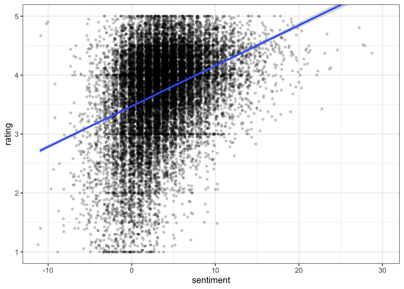

It does appear that there is a positive, probably non-linear relationship between sentiment and rating. We could do some reshaping (normalizing, possibly exponentiating or otherwise transforming the subsequent score) of the sentiment scores to get a better relationship.

beer_data <- 
  beer_data %>%
  mutate(review_id = row_number()) %>%
  left_join(sentiment_ratings)

## Joining, by = "review_id"

beer_data %>%
  select(beer_name, style, rating, sentiment) %>%
  pivot_longer(cols = c(rating, sentiment), names_to = "scale", values_to = "value") %>%
  group_by(style, scale) %>%
  summarize(mean_value = mean(value, na.rm = TRUE),
            se_value = sd(value, na.rm = TRUE) / sqrt(n())) %>%
  group_by(scale) %>%
  slice_max(order_by = mean_value, n = 10) %>%
  ungroup() %>%
  mutate(style = factor(style) %>% reorder_within(by = mean_value, within = scale)) %>%
  ggplot(aes(x = style, y = mean_value, fill = scale)) + 
  geom_col(position = "dodge", show.legend = FALSE) + 
  scale_x_reordered() +
  coord_flip() +
  facet_wrap(~scale, scales = "free")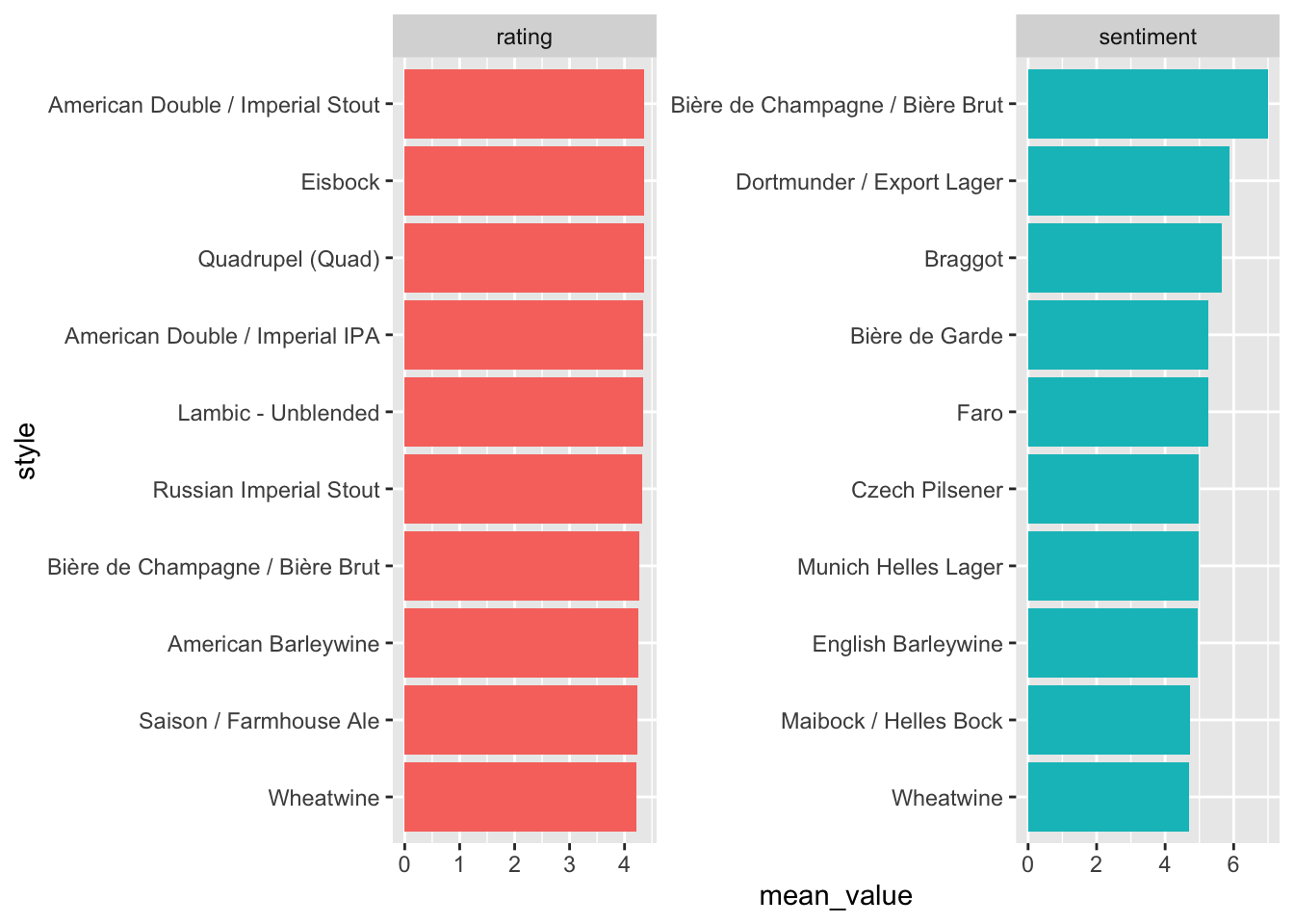

We can see that we get quite different rankings from sentiment scores and from ratings. It might behoove us to examine some of those mismatches in order to identify where they originate from.

# Here are the reviews where the ratings most disagree with the sentiment
beer_data %>%
  # normalize sentiment and ratings so we can find the largest mismatch
  mutate(rating_norm = rating / max(rating, na.rm = TRUE),
         sentiment_norm = sentiment / max(sentiment, na.rm = TRUE),
         diff = rating_norm - sentiment_norm) %>%
  select(review_id, beer_name, sentiment_norm, rating_norm, diff, cleaned_review) %>%
  slice_max(order_by = diff, n = 2) %>%
  gt::gt()

review_id	beer_name	sentiment_norm	rating_norm	diff	cleaned_review
16065	Imperial Stout	-0.3448276	0.980	1.324828	: The color is of black paint. The charcoal-brown head disappears quickly. The smell is of bitterness. Deep, unabiding bitterness of tortured souls. Peets espresso Burning pine forests Sticky, toung-lashing bitterness with a monster grip forces flavors of dried fig, cigar, hazelnut and bitter chocolate (i.e. Valrhona percent Guanaja ). This is a big, big beer. Not for the timid. Primordial, bowels-of-the-earth type energy is packed in to this now larger, oz. bottle.
15808	Adam	-0.3448276	0.974	1.318828	I sampled batch number , I'm gonna put one of these guys away and try it again in a year.Pours syrupy with no head, especially if one follows the directions on the bottle indicating to pour slowly, and I am a sucker for directions on the bottle. Color is incredibly dark brown, completely opaque. Leaves a slight lace as one slowly sips this beer down.Smell is quite complex and sorting it out completely is above the ability of my paltry nose. I would describe it as a sweet and slightly fruity (think figs, raisins). The enigmatic smell seems to call out drink me, and so I listen.Overtones of alcohol do not seem to affect the complex flavor, even though you do feel your BA levels rising as you sip this bad boy down. It seems the smell did not lie, as the taste of the beer is itself sweet and slightly fruity (again I'm thinking of figs and raisins), but there seems to be even more to sort out. There is a bitterness which comes initially and seems to be countered immediately by the sweet flavor described earlier. Finally, at the end of the sip one nutty and coffee flavors resonate and the mild bitterness is back.Overall:Easily the most drinkable double digit ABV beer I have had. Not for beginners, like Stone Arrogant Bastard, this beer just wants to kick your ass. My suggestion is to let it.

# And here are the reviews where the sentiment most disagreed with the rating
beer_data %>%
  # normalize sentiment and ratings so we can find the largest mismatch
  mutate(rating_norm = rating / max(rating, na.rm = TRUE),
         sentiment_norm = sentiment / max(sentiment, na.rm = TRUE),
         diff = sentiment_norm - rating_norm) %>%
  select(review_id, beer_name, sentiment_norm, rating_norm, diff, cleaned_review) %>%
  slice_max(order_by = diff, n = 2) %>%
  gt::gt()

review_id	beer_name	sentiment_norm	rating_norm	diff	cleaned_review
1477	Harvest Ale (Limited Edition)	1.0000000	0.874	0.1260000	Bottle reviews (JAN) Another nice bier to warm up with on a cold, snowy night! Label states st December . Bottling date, or brew date? Anyhow, label also states best before Nov . Oooops, just a bit late. Oh well. Better nate than lever Into the snifter she goes, and it's a dark brown, opaque brew, with a very thin, wispy head congregating only around the rim of the glass. Upon closer inspection, with a little light turned on, I see that the Harvest has a deep ruby hue. Quite nice! Nose is a potent, sweet, rich combo of dark fruit and malty sweetness. Mmmm! Body is more than medium, almost chewy, and silky smooth. Oh yeah! And the flavor is replete with fruity notes, like plum and raisin. Not quite as sweet as the nose suggests, but bulging with dark fruit notes. The high abv is oh-so-well concealed! Don't feel any real warmth, though it's early yet! Along with the fruit is an undercurrent of caramel/toffee sweetness. Real nice! Gotta sip it though; take your time! Tasty bier!! overall: .appearance: \| smell: . \| taste: . \| mouthfeel: . \| drinkability: * Bottle (FEB) This is a ml bottle of vintage. Poured a very rich, dark brown color, with little transparency to it. Head is a finely bubbled, tan layer, with more head ringing the outer rim of the snifter. It leaves a fair amount of lace, yet nothing spectacular. Upon taking a whiff I am inundated by raisiny, dark fruit aromas, as well as the unmistakable nose of alcohol. Sweet and rich quite nice! The body is medium to medium-plus, and the biers' passage across the tongue ruffles nary a feather nice and smooth! The taste itself is loaded with creamy, rich, sweet flavors lots of dark fruit and some toffee notes as well. A verrry nice sipping bier, which has aged well since '. Cheers!! (././././. = .) *Cask sample from MAY This beer was sampled at the Boston Beer Summit. The following, courtesy of Matthias Neidhart of B. Unite tongue sticking out It was vintage , . percent alc./vol. The wooden cask was primed with E.Dupont'scalvados from Normandie,France, prior to its filled with JW Lees Harvest Ale. Lovely mahogany-like color; minimal head and lace, though. Assertive sweet nose, with alcohol quite present. Very nice body, and the smoothness caresses the tongue. Rich, sweet, malty, oaky, nutty flavors with the ever-present alcohol. A wonderful brew! (././././. = .)
16339	XS Old Crustacean	0.7931034	0.686	0.1071034	Vintage: This is likely a legend in the making, but it is only at AA ball right now. Like any prospect, it needs time to develop, but many of the skills are already in place.Muddy brown-orange. Frothy, creamy khaki head retains well for a brew of this size.Aroma is big on hops, with pine being the dominate persuasion. Some toffee and chocolate hues are noted as well. Taste is, in a word, raw. Ragged, piney hops seem to pierce through everything. Bitterness is huge. Toastedness and chocolate stuggle for survival. There is a solid carmel/toffee base, but this cannot weather the hop melee. Solvent-like alcohol pops up late, forming an oppresive alliance. Faint dark fruits, and perhaps even tropical fruits linger in the distance, too frightened to approached due to the menacing regime. In a year or two (or five), the malts will begin to win this war, and make this much more balanced. But the hops and alcohol are too aggressive at this point to make any headway. The body is in place, smooth and viscious. Chewable, if somewhat syrup-like.Presently, it is only drinkable to witness the carnage. I'd suggest giving this some time to achieve stability. Psychotic hopheads excluded.With some rounding, this will be in the majors someday. A rough diamond as it is, but capable of aspiring to it's big brother. The bigger frame (oz vs oz) helps.Thanks, Bighuge. But I should have let this one develop. Hope to find another one to cellar.-- Vintage: I am truely stunned by this amazing beverage where to start? How about the f'king oz's I want oz bottles But at least I have heard the latest batch comes in them.This is my favorite Barleywine. Fantastic integration after years but this could go strong for several more. Flavor upon flavor. Malt lays down some sweet carmel and (slightly) bready notes. The hops jump on top with some piney and splendedly bitter tones. I also detected some minty hues as well. Sweetness dominates, but in a lovely way. Balance is extraordinary. My lord, is this good.Only drawback (as previously mentioned) is the dollar . for a oz bottle. But still unquestionably worth it. One of the absolute best. Bargain at any price.I am amazed that I can still find this batch, but it is still available in stores in the Madison area. I won't say which ones out of selfishness so you better act fast!!(note to self: pick up more bottles of Ol Crust tomorrow)

Interestingly, we see here some evidence that some kind of normalization for review length might be necessary. Let’s take one more look into this area:

beer_data %>%
  mutate(word_count = tokenizers::count_words(cleaned_review)) %>%
  select(review_id, rating, sentiment, word_count) %>%
  pivot_longer(cols = c(rating, sentiment)) %>%
  ggplot(aes(x = word_count, y = value, color = name)) + 
  geom_jitter() + 
  geom_smooth(method = "lm", color = "black") + 
  facet_wrap(~name, scales = "free") +
  theme_bw() + 
  theme(legend.position = "none")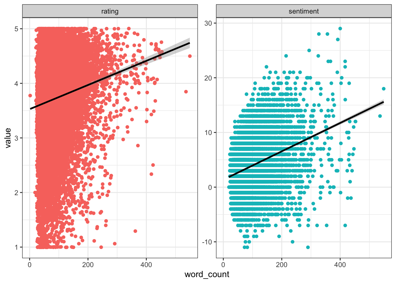

It appears that both rating and sentiment are positively correlated with word count, but that (unsurprisingly) sentiment is more strongly correlated. Going forward, we might want to consider some way to normalize for word count in our sentiment scores.

5.4 Text Analysis Pt. IV: n-gram models

An obvious and valid critique of sentiment analysis as implemented above is the focus on single words, or unigrams. It is very clear that English (and most languages) have levels of meaning that go beyond the single word, so focusing our analysis on single words as are tokens/observations will lose some (or a lot!) of meaning. It is common in modern text analysis to look at units beyond the single word: bi-, tri-, or n-grams, for example, or so-called “skipgrams” for the popular and powerful word2vec family of algorithms. Tools like convolutional and recursive neural networks will look at larger chunks of texts, combined in different ways.

Let’s take a look at bigrams in our data-set: tokens that are made up of 2 adjacent words. We can get them using the same unnest_tokens() function, but with the request to get token = "ngrams" and the number of tokens set to n = 2.

beer_bigrams <- 
  beer_data %>%
  unnest_tokens(output = bigram, input = cleaned_review, token = "ngrams", n = 2)

beer_bigrams %>%
  filter(review_id == 1) %>%
  select(beer_name, bigram)

## # A tibble: 115 × 2
##    beer_name           bigram    
##    <chr>               <chr>     
##  1 Caffrey's Irish Ale this is   
##  2 Caffrey's Irish Ale is a      
##  3 Caffrey's Irish Ale a very    
##  4 Caffrey's Irish Ale very good 
##  5 Caffrey's Irish Ale good irish
##  6 Caffrey's Irish Ale irish ale 
##  7 Caffrey's Irish Ale ale i'm   
##  8 Caffrey's Irish Ale i'm not   
##  9 Caffrey's Irish Ale not sure  
## 10 Caffrey's Irish Ale sure if   
## # … with 105 more rows
## # ℹ Use `print(n = ...)` to see more rows

We can see that, in this first review, we already have a bigram with strong semantic content: not sure should tell us that looking only at the unigram sure will give us misleading results.

We can use some more tidyverse helpers to get a better idea of the scale of the problem. The separate() function breaks one character vector into multiple columns, according to whatever separating characters you specify.

beer_bigrams %>%
  separate(col = bigram, into = c("word1", "word2"), sep = " ") %>%
  # Now we will first filter for bigrams starting with "not"
  filter(word1 == "not") %>%
  # And then we'll count up the most frequent pairs of negated biterms
  count(word1, word2) %>%
  arrange(-n)

## # A tibble: 1,298 × 3
##    word1 word2     n
##    <chr> <chr> <int>
##  1 not   a      1511
##  2 not   as      777
##  3 not   much    709
##  4 not   bad     522
##  5 not   too     473
##  6 not   the     376
##  7 not   quite   310
##  8 not   to      283
##  9 not   very    260
## 10 not   sure    251
## # … with 1,288 more rows
## # ℹ Use `print(n = ...)` to see more rows

We can see that the 4th most frequent pair is “not bad”, which means that bad, classified as a negative token in the sentiments tibble, is actually being overcounted as negative in our simple unigram analysis.

We can actually look more closely at this with just a little bit more wrangling:

beer_bigrams %>%
  separate(col = bigram, into = c("word1", "word2"), sep = " ") %>%
  filter(word1 == "not") %>%
  inner_join(sentiments, by = c("word2" = "word")) %>%
  count(word1, word2, sort = TRUE)

## # A tibble: 303 × 3
##    word1 word2            n
##    <chr> <chr>        <int>
##  1 not   bad            522
##  2 not   enough         111
##  3 not   overwhelming   104
##  4 not   great           90
##  5 not   worth           73
##  6 not   good            65
##  7 not   like            65
##  8 not   outstanding     46
##  9 not   bitter          44
## 10 not   overbearing     43
## # … with 293 more rows
## # ℹ Use `print(n = ...)` to see more rows

We could use such an approach to try to get a handle on the problem of context in our sentiment analysis, by inverting the sentiment score of any word that is part of a “not bigram”. Of course, such negations can be expressed over entire sentences, or even flavor the entire text (as in the use of sarcasm). There are entire analysis workflows built on this kind of context flow.

For example, the sentiment package, which was used in the recent Luc et al. (2020) paper on free JAR analysis, takes just such an approach. We can quickly experiment with this package as a demonstration.

library(sentimentr)

polarity_sentiment <- 
  cleaned_reviews_example %>% 
  select(beer_name, rating, cleaned_review) %>%
  get_sentences() %>%
  sentiment_by(by = "beer_name")

polarity_sentiment

##                   beer_name word_count        sd ave_sentiment
## 1:           Black Bear Ale        119 0.2304159   0.007328644
## 2:                    Kozel        187 0.2651420   0.306529868
## 3: Odell Cutthroat Pale Ale         45 0.5829988   0.435923231
## 4:         Pike XXXXX Stout        102 0.2946472  -0.027863992
## 5:          Stoudt's Weizen         46 0.2081545   0.155677045

We can visualize how the sentimentr algorithm “sees” the sentences by using the highlight(polarity_sentiment) call, but since this outputs HTML I will embed it as an image here.

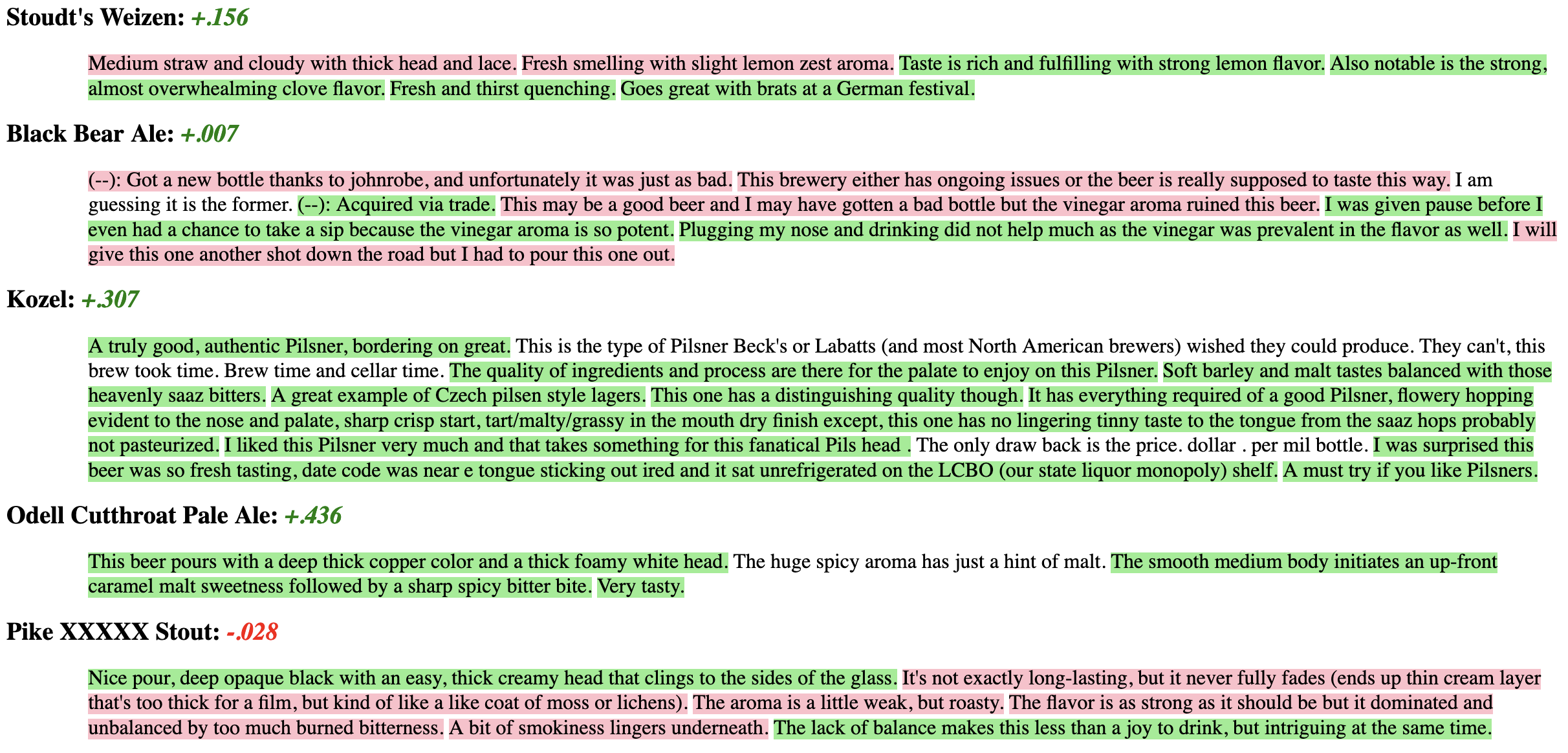
sentimentr sentence-based sentiment analysis, using the dictionary-based, polarity-shifting algorithm.

As a note, this is only one example of such an algorithm, and it may or may not be the best one. While Luc et al. (2020) found good results, we (again plugging our poster) found that sentimentr didn’t outperform simpler algorithms. However, this may have to do with the set up of lexicons, stop-word lists, etc.