1 A crash course in `R`

In this section, we’re going to go over the basics of R: what the heck you’re looking at, how the RStudio IDE works, how to extend R with packages, and some key concepts that will help you work well in R.

1.1 `R` vs RStudio

In this workshop we are going to be learning the basics of coding for text analysis in R, but we will be using the RStudio interface/IDE! Why am I using R for this workshop? And why do we need this extra layer of program to deal with it?

1.1.1 What is `R`?

R is a programming language that was built for statistical and numerical analysis. It is not unique in these spaces–most of you are probably familiar with a program like SAS, SPSS, Unscrambler, XLSTAT, JMP, etc. Unlike these, R is free and open-source. This has two main consequences:

R is constantly being extended to do new, useful things because there is a vibrant community of analysts developing tools for it, and the barrier to entry is very low.
R doesn’t have a fixed set of tasks that it can accomplish, and, in fact, I generally haven’t found a data-analysis task I needed to do that I couldn’t in R.

Because it’s a programming language, R isn’t point-and-click–today we’re going to be typing commands into the console, hitting, enter, making errors, and repeating. But this is a good thing! The power and flexibility of R (and it’s ability to do most of the things we want) come from the fact that it is a programming language. While learning to use R can seem intimidating, the effort to do so will give you a much more powerful suite of tools than the more limited point-and-click alternatives. R is built for research programming (data analysis), rather than for production programming. The only other alternative that is as widely supported in the research community is Python, but–honesty time here–I have never learned Python very well, and so we are learning R. And, in addition, Python doesn’t have as good an Interactive Development Environment (IDE, explained further below) as RStudio!

If you open your R.exe/R application, you’ll see something like this:

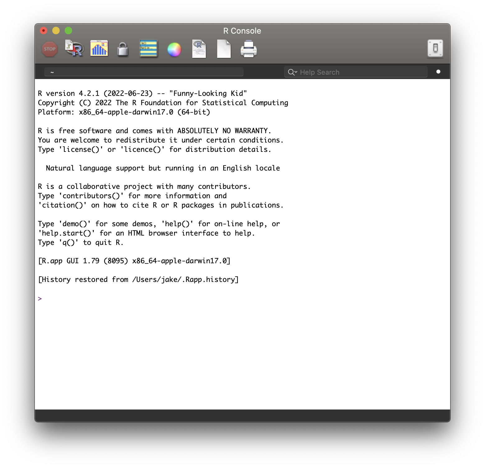
The R graphical console

You can also work with R from a shell interface, but I will not be discussing this approach in this workshop.

1.1.2 Great, why are we using RStudio then?

RStudio is an “Interactive Development Environment” (IDE) for working with R. Without going into a lot of detail, that means that R lives on its own on your computer in a separate directory, and RStudio provides a bunch of better functionality for things like writing multiple files at once, making editing easier, autofilling code, and displaying plots. You can learn more about RStudio here.

With that out of the way, I am going to be sloppy in terminology and say/type “R” a lot of the times I mean “RStudio”. I will be very clear if the distinction actually matters. RStudio is going to make your life way easier, and when you try to learn Python you are going to be sad :(

1.2 The parts of RStudio

The default layout of RStudio looks something like this (font sizes may vary):

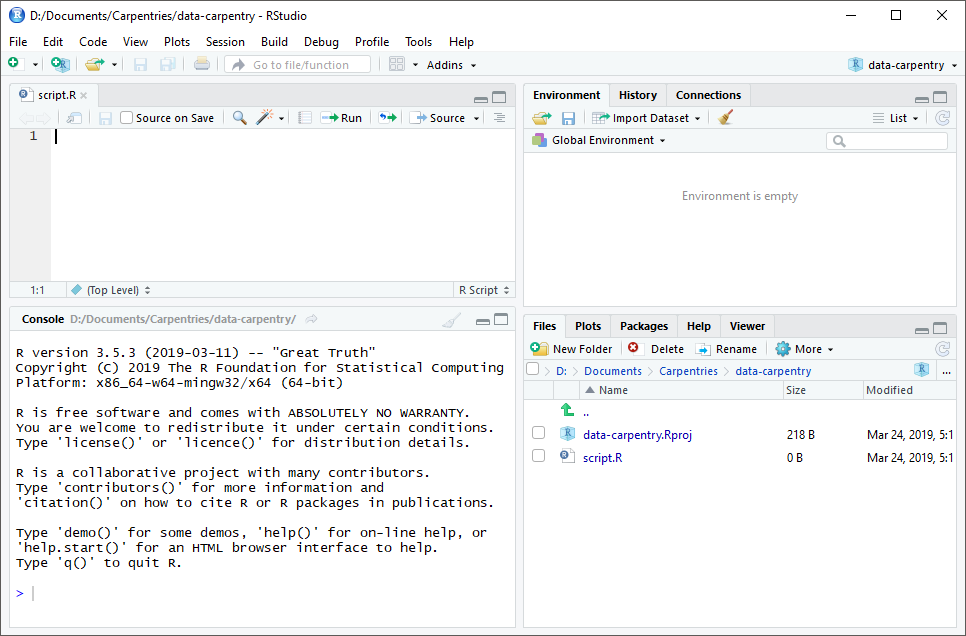
RStudio default layout, courtesy of Data Carpentry

RStudio always has 4 “panes” with various functions, which are in tabs (just like a web browser). The key ones for right now to pay attention are:

The Console tab is the portal to interact directly with R. The > “prompt” is where you can type and execute commands (by hitting return). You can try this out right now by using it like a calculator - try 1 + 1 if you like!
The Files tab shows the files in your working directory: like in the Windows Explorer or macOS Finder, files are displayed within folders. You can click on files to open them.
The Help tab shows documentation for R functions and packages–it is useful for learning how to use specific functions.
The Plots tab shows graphical output, and this is where the data visualizations we’ll learn to make will (generally) appear.
The Environment tab shows the objects that exist in memory in your current R session. Without going into details, this is “what you’ve done” so far: data tables and variables you’ve created, etc.
Finally, the Scripts pane shows individual tabs for each script and other RStudio file. Scripts (and other, more exotic file types like RMarkdown/.Rmd files) are documents that contain multiple R commands, like you’d type into the Console. However, unlike commands in the Console, these commands don’t disappear as soon as they’re run, and we can string them together to make workflows or even programs. This is where the real power of R will come from.

You can change the layout of your Panes (and many other options) by going to the RStudio menu: Tools > Global Options and select Pane Layout.

You’ll notice that my layout for RStudio looks quite different from the default, but you can always orient yourself by seeing what tab or pane I am in–these are always the same. I prefer giving myself more space for writing R scripts and markdown files, so I have given that specific Pane more space while minimizing the History pane.

While we’re in Global Options, please make the following selections:

Under General, uncheck all the boxes to do with restoring projects and workspaces. We want to make sure our code runs the same time every time (i.e., that our methods are reproducible), and letting RStudio load these will make this impossible:

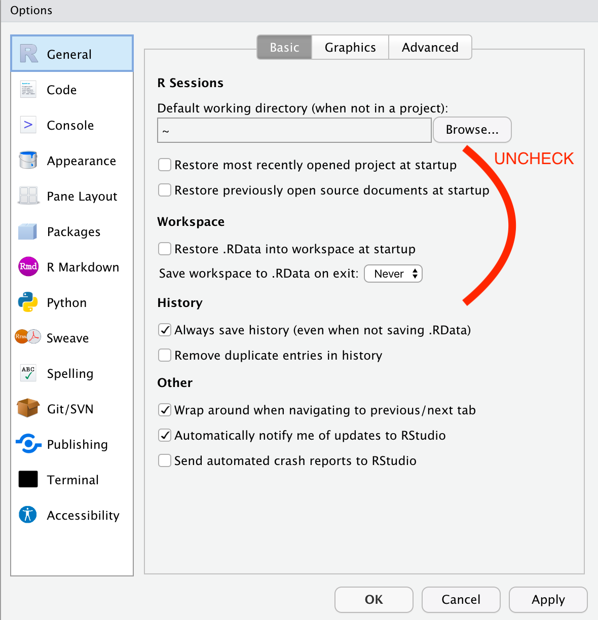
Uncheck the options to restore various data and projects at startup.

Make your life easier by setting up autocompletion for your code. Under the Code > Completion options, select the checkboxes to allow using tab for autocompletions, and also allowing multiline autocompletions. This means that RStudio will suggest functions and data for you if you hit tab, which will make you have to do way less typing:

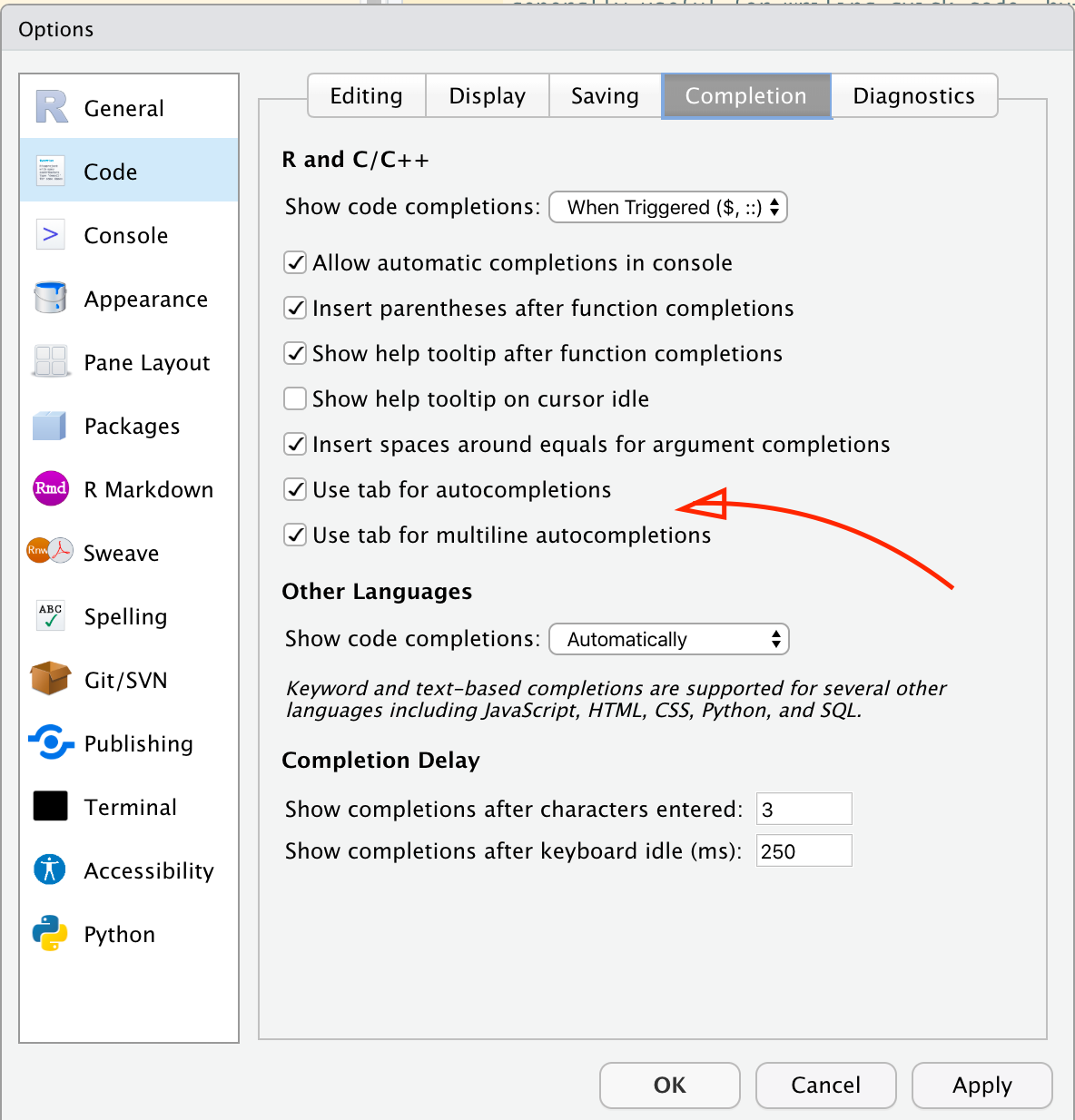
Check the boxes for tab and multiline autocompletions.

1.2.1 The “working directory” and why you should care

Before we move on to using R for real, we have one key general computing concept to tackle: the “working directory”. The working directory is the folder on your computer in which R will look for files and save files. When you need to tell R to read in data from a file or output a file, you will have to do so in relation to your working directory. Therefore, it is important that you know how to find your working directory and change it.

The easiest (but not best) way to do this is to use the Files pane. If you hit the “gear” icon in the Files pane menu, you’ll see two commands to do with the working directory. You can Go To Working Directory to show you whatever R currently has set as the working directory. You can then navigate to any directory you want on your hard drive, and use the Set As Working Directory command to make that the working directory.

A better way to do this is to use the R commands getwd() and setwd().

getwd() # will print the current working directory

## [1] "/Users/jake/Dropbox/Work/Documents/Conferences/Eurosense 2022/Sensometrics Tutorial/eurosense-tutorial-2022"

And we can manually change the working directory by using

setwd("Enter/Your/Desired/Directory/Here")

Notice that I am not running the second command, because it would cause an error!

When we use R to navigate directories, I recommend always using the forward slash: /, even thouhg on Windows systems the typical slash is the backslash: \. R will properly interpret the / for you in the context of your operating system, and this is more consistent with most modern code environments.

1.3 Extending `R` with packages

One of the key advantages of R is that its open-source nature means that you can extend it to do all sorts of things. For example, for much of this workshop we are going to be going about basic text analysis using the tidytext package. There are various ways to install new packages, but the easiest way is to use the Packages tab. This will show you all the packages you currently have installed as an alphabetical list.

1.3.1 Installing packages

To install a new package, you can select the Install button from the Packages tab, which will give you a prompt to type the package name in. You can get to the same prompt by going to the Tools > Install Packages... menu. On this prompt, you can list packages separated by a comma (,), which is convenient. RStudio will also try to help you by autocompleting package names.

You should have already installed the tidyverse package as part of your pre-work for this workshop. Now, let’s go ahead and install the tidytext package, which we’ll use later in this workshop. If you didn’t install the tidyverse package, you can list it along with the tidytext package.

You’ll note that hitting Install made a line of code appear in your console, something like:

install.packages("tidytext")

This is the “true” R way to install packages–the function install.packages() can be run on the Console to install whatever package is quoted inside the parentheses.

You can get R packages from a variety of sources. The most common are repositories, like CRAN, which is where you first downloaded R. There are others, like Bioconductor, which is used more by the bioinformatics community. You might also sometime download an install a package that isn’t on a repository, such one from github (for example this one), but I am not going to cover that in detail here.

1.3.2 Loading packages

To actually use a package, you need to load it using the library(<name of package>) command. So, for example, to load the tidyverse package we will use the command

library(tidyverse)

You need to use multiple library() commands to load multiple packages, e.g.,

library(tidyverse)
library(tidytext)

If you want to know what packages you have loaded, you can run the sessionInfo() function, which will tell you a bunch of stuff, including the “attached” packages:

sessionInfo()

## R version 4.2.1 (2022-06-23)
## Platform: x86_64-apple-darwin17.0 (64-bit)
## Running under: macOS Catalina 10.15.7
## 
## Matrix products: default
## BLAS:   /Library/Frameworks/R.framework/Versions/4.2/Resources/lib/libRblas.0.dylib
## LAPACK: /Library/Frameworks/R.framework/Versions/4.2/Resources/lib/libRlapack.dylib
## 
## locale:
## [1] en_US.UTF-8/en_US.UTF-8/en_US.UTF-8/C/en_US.UTF-8/en_US.UTF-8
## 
## attached base packages:
## [1] stats     graphics  grDevices utils     datasets  methods   base     
## 
## other attached packages:
##  [1] tidytext_0.3.3  forcats_0.5.1   stringr_1.4.0   dplyr_1.0.9    
##  [5] purrr_0.3.4     readr_2.1.2     tidyr_1.2.0     tibble_3.1.7   
##  [9] ggplot2_3.3.6   tidyverse_1.3.2
## 
## loaded via a namespace (and not attached):
##  [1] Rcpp_1.0.9          lattice_0.20-45     lubridate_1.8.0    
##  [4] assertthat_0.2.1    digest_0.6.29       utf8_1.2.2         
##  [7] R6_2.5.1            cellranger_1.1.0    backports_1.4.1    
## [10] reprex_2.0.1        evaluate_0.15       httr_1.4.3         
## [13] pillar_1.8.0        rlang_1.0.4         googlesheets4_1.0.0
## [16] readxl_1.4.0        rstudioapi_0.13     jquerylib_0.1.4    
## [19] Matrix_1.4-1        rmarkdown_2.14      googledrive_2.0.0  
## [22] bit_4.0.4           munsell_0.5.0       broom_1.0.0        
## [25] janeaustenr_0.1.5   compiler_4.2.1      modelr_0.1.8       
## [28] xfun_0.31           pkgconfig_2.0.3     htmltools_0.5.3    
## [31] tidyselect_1.1.2    bookdown_0.27       fansi_1.0.3        
## [34] crayon_1.5.1        tzdb_0.3.0          dbplyr_2.2.1       
## [37] withr_2.5.0         SnowballC_0.7.0     grid_4.2.1         
## [40] jsonlite_1.8.0      gtable_0.3.0        lifecycle_1.0.1    
## [43] DBI_1.1.3           magrittr_2.0.3      tokenizers_0.2.1   
## [46] scales_1.2.0        vroom_1.5.7         cli_3.3.0          
## [49] stringi_1.7.8       cachem_1.0.6        fs_1.5.2           
## [52] xml2_1.3.3          bslib_0.4.0         ellipsis_0.3.2     
## [55] generics_0.1.3      vctrs_0.4.1         tools_4.2.1        
## [58] bit64_4.0.5         glue_1.6.2          hms_1.1.1          
## [61] parallel_4.2.1      fastmap_1.1.0       yaml_2.3.5         
## [64] colorspace_2.0-3    gargle_1.2.0        rvest_1.0.2        
## [67] knitr_1.39          haven_2.5.0         sass_0.4.2

Finally, you can also load (and unload) packages using the Packages tab, by clciking the checkbox next to the name of the package you want to load (or unload).

1.4 Getting help

With more packages you’re going to more frequently run into the need to look up how to do things, which means dealing with help files. You can always get help on a particular function by typing ?<search term>, which will make the help documentation for whatever you’ve searched for appear.

For example, try typing the following to get help for the sessionInfo() command:

?sessionInfo

But what if you don’t know what to search for?

By typing ??<search term> you will search all help files for the search term. R will return a list of matching articles to you in the help pane. This is considerably slower, since it’s searching hundreds or thousands of text files. Try typing ??install into your console to see how this works.

You will notice that there are two types of results in the help list for install. The help pages should be familiar. But what are “vignettes”? Try clicking on one to find out.

Vignettes are formatted, conversational walkthroughs that are increasingly common (and helpful!) for R packages. Rather than explaining a single function they usually explain some aspect of a package, and how to use it. And, even better for our purposes, they are written in R Markdown. Click the “source” link next to the vignette name in order to see how the author wrote it in R Markdown. This is a great way to learn new tricks.

While you can find vignettes as we just did, a better way is to use the function browseVignettes(). This opens a web browser window that lists all vignettes installed on your computer. You can then use cmd/ctrl + F to search using terms in the web browser and quickly find package names, function names, or topics you are looking for.

1.5 Livecoding along

We’ve now covered the Console tab and the Scripts pane. These are both areas in which you can write and execute code, but they work a little differently. The Console is the place to run code that is short and easy to type, or that you’re experimenting with. It will allow you to write a single line of code, and after you hit return, R will execute the command. This is great for “interactive programming”, but it isn’t so great for building up a complex workflow, or for following along with this workshop!

This is why I have recommended that you create a new script to follow along with this workshop. Again, you get a new script by going to File > New File > R Script. You can write multiple lines of code and then execute each one in any order (although keeping a logical sequence from top to bottom will help you keep track of what you’re doing). In an R script, everything is expected to be valid R code.

You can't write this in an R script because it is plain text.  This will
cause an error.

# If you want to write text or notes to yourself, use the "#" symbol at the start of 
# every line to "comment" out that line.  You can also put "#" in the middle of
# a line in order to add a comment - everything after will be ignored.

1 + 1 # this is valid R syntax

print("hello world") # this is also valid R syntax

To run code from your R script, put your cursor on the line you want to run and either hit the run button with the green arrow at the top left or (my preferred method) type cmd + return (on Mac) or ctrl + return (on PC).

1 A crash course in R

1.1 R vs RStudio

1.1.1 What is R?